 Gustav
 Abstract
We study four tiny plain convolutional networks with 1, 2, 4, and 8 conv layers of 16 channels on downsampled Fashion-MNIST. The task is to fit a fixed set of 10,000 training images, so the measure of success is final training cross-entropy; held-out accuracy is reported only as a secondary check. We compare a fixed LeakyReLU–LayerNorm–3×3 recipe, a search over one shared activation/normalization/kernel choice, and independent choices in every layer. Each search includes the default and receives up to 32 candidate fits. Three independent search repetitions select configurations using training loss; each selected configuration is then retrained with three fresh seeds. We record 416 unique search fits and 171 fresh-seed assessment fits, with additional learning-rate and training-horizon controls. Unlike an earlier fully connected attempt, depth helped here: the default network's fit to the training set improved from 1 to 4 layers (training cross-entropy 0.498, 0.400, 0.190) and then stalled at 8 layers (0.203). Architectural tuning improved the fit by 7% at 1 layer, 14% at 2, 50% at 4 and 36% at 8 (per-layer search, up to 32 trials), so in this setting the benefit of tuning grew strongly with depth, though not monotonically, and every one of the twelve per-layer searches beat its default. Shallow networks obtained nearly all of their gain within 4-8 trials, while the 4- and 8-layer searches were still improving at 16-32 trials. A twelve-configuration shared recipe (almost always GELU + LayerNorm + 5x5 kernels) matched or beat per-layer search at 1-4 layers for roughly 40% of the compute; per-layer search led only at 8 layers. Two controls support the reading: a learning-rate-only search helped most at 1 layer and little at 4-8 layers, and the selected architectures kept their advantage when trained for 40 epochs. Important caveats: the winning recipes have about 2 times more parameters than the default, so part of the gain is added capacity; the gains in training fit barely carry over to held-out accuracy at 4-8 layers; and each cell rests on three searches. These findings describe a small, fixed-width, fixed-split experiment; they do not establish a universal depth-scaling law.
What we found
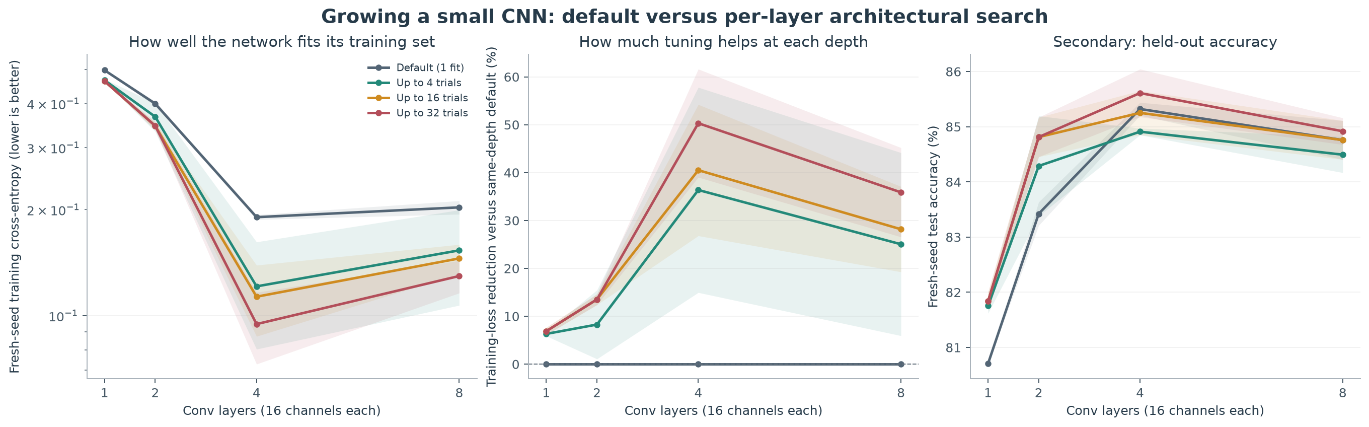
- Depth helped fitting, up to a point. Default training cross-entropy fell from 0.498 (1 layer) to 0.400 (2) to 0.190 (4), then did not improve at 8 layers (0.203). Even tuned, 8 layers fit worse than 4 (0.130 versus 0.095 for per-layer search at 32 trials), so with plain layers, width 16 and 20 epochs the useful depth ends near 4.
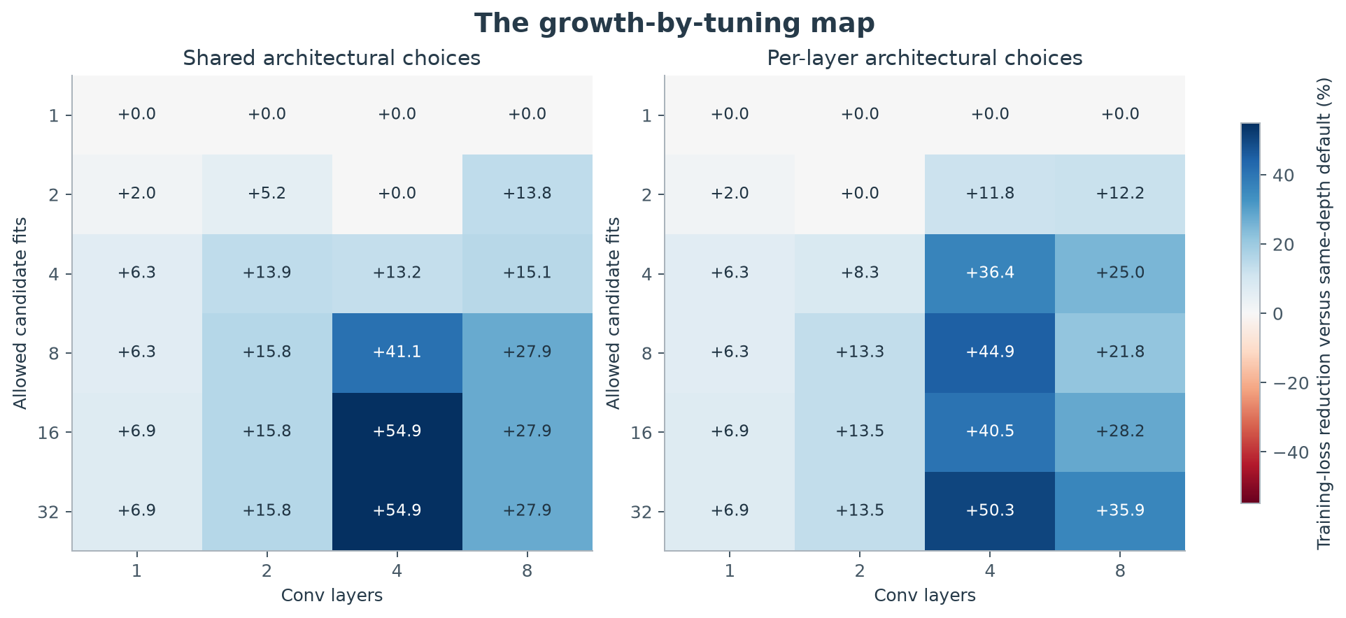
- Tuning mattered more as the network grew. The reduction in training loss versus the same-depth default, for per-layer search with up to 32 trials, was 6.9%, 13.5%, 50.3% and 35.9% at 1, 2, 4 and 8 layers. All twelve searches (4 depths x 3 repetitions) improved on the default; the individual repetitions were 6-8% at 1 layer, 12-15% at 2, 37-58% at 4 and 30-47% at 8, so the 1-2 layer and 4-8 layer ranges do not overlap.
- Deeper networks needed more search attempts. At 1 and 2 layers the per-layer curve was within 10% of its final gain after 4 and 8 trials (6.3% of 6.9%; 13.3% of 13.5%). At 4 layers it kept rising to 50% at 32 trials and at 8 layers it was still climbing (25% at 4 trials, 28% at 16, 36% at 32).
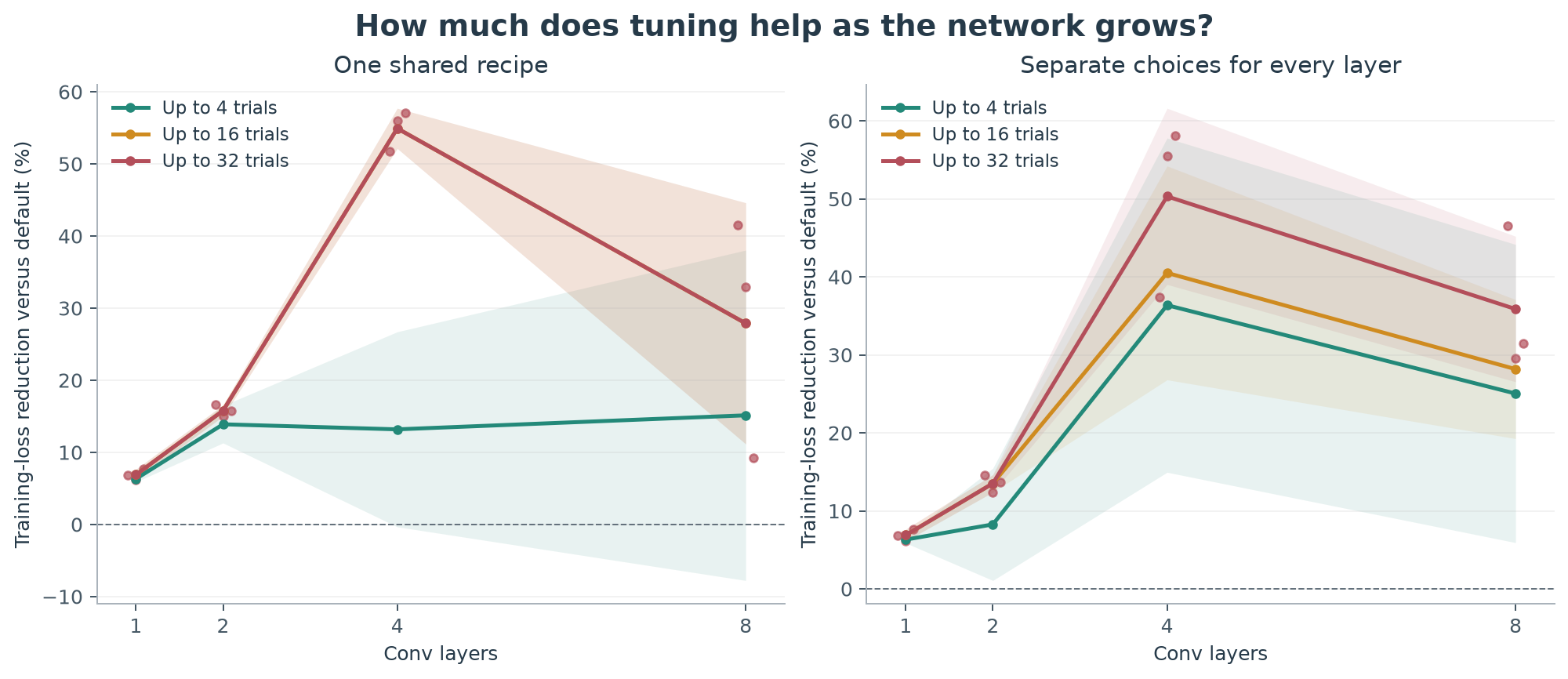
- A small shared recipe captured most of the benefit cheaply. Trying twelve uniform recipes (one choice repeated at every layer) reduced training loss by 6.9%, 15.8%, 54.9% and 27.9%; GELU + LayerNorm + 5x5 won 11 of 12 shared searches. Per-layer search was no better at 2 and 4 layers and cost about 2.6 times more CPU time. It led only at 8 layers (35.9% versus 27.9%), where the shared result varied a lot between repetitions (9% to 42%).
- Depth bought more than tuning at shallow depth. The untuned 4-layer network (0.190, 42 CPU-s to train) fit better than any tuned 1- or 2-layer network, including the 32-trial per-layer search at 2 layers (0.346, 1,034 CPU-s).
- The normalization choice was the dominant lever and its importance grew with depth. Averaged over the twelve shared recipes, networks without LayerNorm had training loss 1.14 times (1 layer), 1.30 times (2), 2.27 times (4) and 2.20 times (8) that of networks with it. The default already had LayerNorm; the tuned gains came mainly from GELU and the larger kernel.
- Part of the gain is added capacity. The shared winners had 1.2, 2.1, 2.4 and 2.6 times the parameters of the default at 1, 2, 4 and 8 layers (per-layer winners 1.2, 2.1, 2.3 and 1.8 times), because 5x5 kernels have 2.8 times the weights of 3x3 kernels. This study cannot separate better design from more parameters.
- Gains in fitting the training set mostly did not carry over to held-out accuracy at depth. Test accuracy with per-layer tuning rose by about 1.1 and 1.4 percentage points at 1 and 2 layers but only by 0.3 and 0.2 points at 4 and 8 layers, exactly where the training-loss gains were largest.
- Two checks held up. A three-value learning-rate search recovered 12.7%, 8.0% and 0% at 1, 4 and 8 layers, more than architecture search at 1 layer but far less at 4 and 8 layers. Retraining the selected architectures for 40 epochs kept (and, in relative terms, enlarged) their advantage: 79% and 52% lower training loss than the default at 4 and 8 layers for per-layer selections.
1The experiment
Growth means separately training networks with more conv layers from scratch. We do not append layers to a trained model or transfer weights. Each block is Conv(16 channels, same padding) → optional affine LayerNorm (a one-group GroupNorm) → activation; 2×2 max-pooling follows blocks 1 and 3 when they exist, then average pooling to 3×3 and a linear classifier predict ten classes. There are no residual connections, dropout, or data augmentation. The objective is to fit a fixed 10,000-image training set; we deliberately do not tune for generalization, so overfitting is not penalized.
Why this replaces an earlier attempt. A first version used fixed-width 16-unit fully connected networks. There, adding layers made fitting and generalization worse, which does not match the common experience that depth helps and made the tuning question hard to interpret. That earlier run is not part of the findings below; we mention it so that the choice of a CNN is not hidden.
| Quantity | Executed setting |
|---|---|
| Data | Fashion-MNIST; 2 × 2 average pooling to 14 × 14 pixels |
| Fitted set | 10,000 training images (1,000 per class), fixed; 6,000 validation images unused for selection; 10,000 official test images used only for the secondary accuracy |
| Normalization | One pixel mean and standard deviation estimated from training data only |
| Depth and width | 1, 2, 4, 8 conv layers; 16 channels |
| Default parameter count | 1,642 at depth 1; 18,106 at depth 8 |
| Choices per layer | Activation ReLU / LeakyReLU(0.01) / GELU × normalization none / LayerNorm × kernel 3 / 5 = 12 |
| Training | Adam, learning rate 0.001, batch 128, 20 epochs; selection on final-epoch training cross-entropy |
| Budget checkpoints | 1, 2, 4, 8, 16, 32 candidate fits, including the default |
| Replication | 3 independent search repetitions; 3 fresh training seeds per selected configuration |
| Compute | Five CPU workers, one PyTorch thread each; per-fit process CPU time recorded |
Layers use PyTorch's default initialization for every activation; normalization starts with unit scale and zero offset. The pooling placement and spatial head were chosen from default-network pilot runs, so that fitting improves with depth, before the main search; the 20-epoch horizon bounds compute, and a separate 40-epoch check measures whether selected configurations retain their advantage with longer training. The exact executed settings are recorded in protocol.json; the earlier design note is a proposal, not a substitute for that record.
Shared versus per-layer tuning
Shared search has twelve configurations at every depth: one activation/normalization/kernel triple is repeated throughout the network. Per-layer search has 12^d configurations at depth d, reaching about 430 million at eight layers. It starts from the same fixed default, then samples uniformly without replacement. Shared search similarly starts with the default and randomly orders the other eleven choices. At depth one the spaces and search orders are identical. Search stops when a space is exhausted; later budget checkpoints retain its incumbent.
Search orders are generated in advance; all requested candidates are run in a shuffled execution order to distribute changing background load. Fits appearing in both arms are reused, while each arm is charged the cost it would incur alone. Larger budgets are prefixes of the same search, not independent restarts. We select the lowest final training cross-entropy, breaking ties by first occurrence. Protocol and search hashes are stored with the frozen selections before final test evaluation.
Exhausting twelve shared architectures does not eliminate training-seed uncertainty. This protocol spends the search budget on distinct configurations and does not use the remaining allowance to repeat their training seeds. It therefore compares two architecture-sampling strategies, rather than the best possible allocation of all available compute.
2Hypotheses and what would change our minds
| Hypothesis | Evidence sought | Version 2.0 assessment |
|---|---|---|
| H1. Tuning becomes more valuable as the network grows. | The improvement over the same-depth default grows with depth at a fixed search budget. | Supported in this setting, with a caveat. Relative training-loss reduction at 32 trials: 6.9%, 13.5%, 50.3%, 35.9% at 1, 2, 4, 8 layers; all twelve searches improved and the shallow and deep ranges do not overlap. It is not monotone (8 layers below 4), and part of the growth is headroom: the default stalls at 4-8 layers. Part is added capacity from 5x5 kernels. |
| H2. Per-layer freedom needs a larger budget before it pays; shared tuning wins early. | Shared search leads at small budgets; per-layer overtakes it later, with the crossover moving right with depth. | Weak support. Per-layer search was ahead of the shared recipe only at 8 layers and only at 32 trials (0.130 versus 0.146, with three repetitions and a very variable shared result). At 2 and 4 layers the twelve-configuration shared search matched or beat it at about 40% of the cost. A single crossover point cannot show how the crossover moves with depth. |
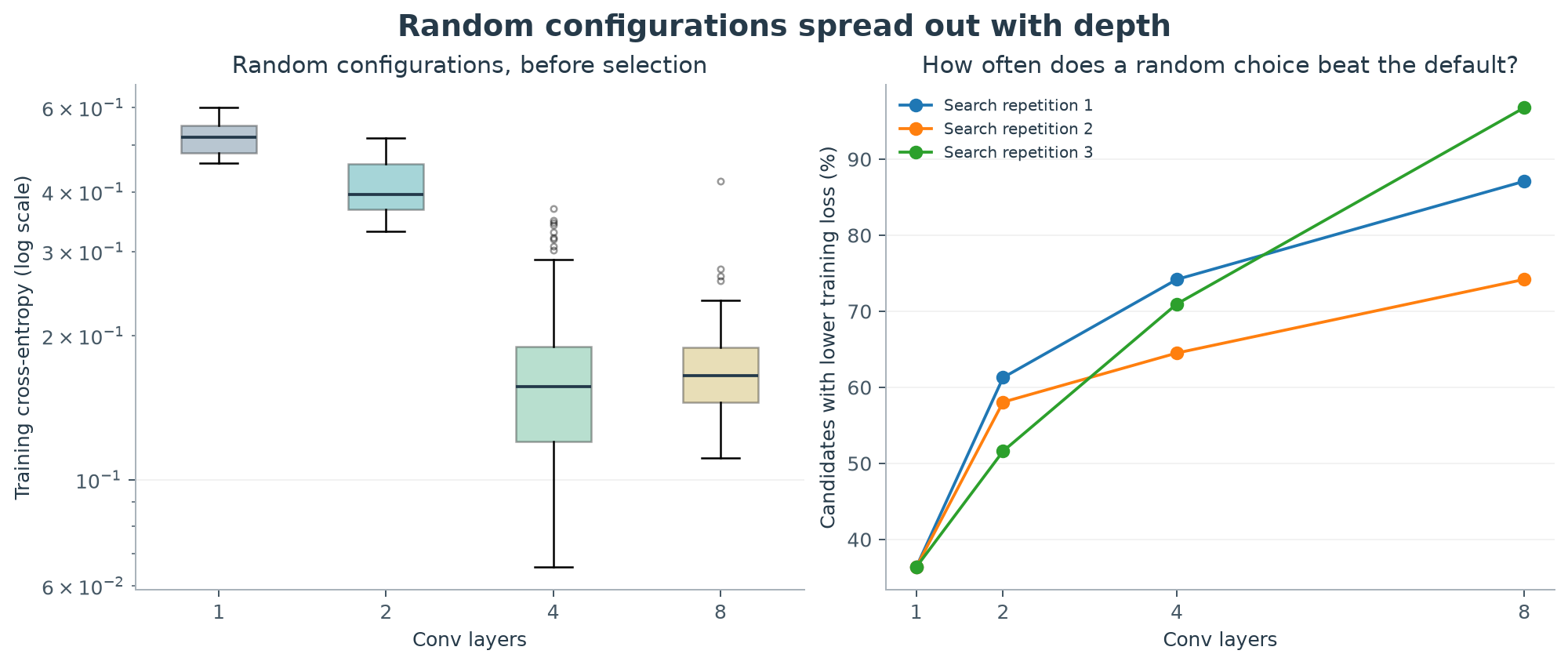
| H3. Good configurations become rarer with depth. | Random configurations increasingly train poorly; a small fraction beats the default. | Not supported. The fraction of random per-layer candidates that beat the default rose with depth: 36%, 57%, 70% and 86% at 1, 2, 4, 8 layers. The spread of outcomes widened (best-to-worst training loss 0.46-0.60 at 1 layer, 0.07-0.37 at 4, 0.11-0.42 at 8), but the default itself stalled, so what grew was headroom, not rarity. |
| H4. The best depth depends on the tuning compute available. | Shallow tuned networks win at small budgets; deeper networks overtake with more search. | Not supported. The best depth was 4 at every budget we measured, and the untuned 4-layer network beat every tuned 1- and 2-layer network. Depth 8 never overtook depth 4 within 20 epochs. |
A larger tuning gain can arise because the best model improves, because the default worsens, or both. We therefore report absolute accuracy and loss alongside improvement over the default at the same depth. The comparison of shared and per-layer search also changes the sampling prior: homogeneous configurations are common in shared search and rare in uniform per-layer search. It evaluates two practical search designs, not a pure causal intervention on dimensionality alone.
3How tuning changes the growth curve
| Layers | Default training loss | Shared, ≤32 trials | Per-layer, ≤32 trials | Per-layer reduction (%) | Default test acc. (%) | Per-layer test acc. (%) |
|---|---|---|---|---|---|---|
| 1 | 0.498 ± 0.004 | 0.463 ± 0.002 | 0.463 ± 0.002 | +6.9 | 80.71 ± 0.01 | 81.84 ± 0.17 |
| 2 | 0.400 ± 0.006 | 0.337 ± 0.008 | 0.346 ± 0.009 | +13.5 | 83.42 ± 0.21 | 84.81 ± 0.36 |
| 4 | 0.190 ± 0.003 | 0.086 ± 0.006 | 0.095 ± 0.022 | +50.3 | 85.32 ± 0.12 | 85.61 ± 0.43 |
| 8 | 0.203 ± 0.009 | 0.146 ± 0.030 | 0.130 ± 0.014 | +35.9 | 84.76 ± 0.35 | 84.92 ± 0.24 |
Values are means ± descriptive SD across the three independent search repetitions after averaging fresh training seeds within each repetition. Percentage reductions are paired against the same-depth default. Small differences should not be read as statistically established effects. Training cross-entropy (fit to the fixed set) is the primary metric; held-out accuracy is a secondary diagnostic and was never used for selection.
Reading Figure 1 left to right: the default curve falls steeply to 4 layers and then flattens, while the tuned curves fall further and keep the same shape. The middle panel is the main picture you asked for: the benefit of tuning rises from under 10% at one layer to removing about half of the training loss at four layers, and stays large (about a third) at eight. Because absolute losses shrink with depth, the percentage reduction is the fairer measure, and the absolute values are in the table.
The decline from 4 to 8 layers should not be over-read. At eight layers the results varied much more between repetitions (per-layer: 47%, 30%, 32%; shared: 42%, 33%, 9%), so the evidence for 'tuning helps less at 8 than at 4' is weaker than the evidence for 'tuning helps much more at 4-8 than at 1-2'.
Tuning also changed which depth looks attractive: the default 8-layer network is no better than the default 4-layer network, but a tuned 8-layer network (0.130) is clearly better than the default 4-layer one (0.190). Whether depth helps therefore depends on whether the deeper network is tuned, though a tuned 4-layer network (0.095) still wins in this setup.
4How many attempts—and how much compute?
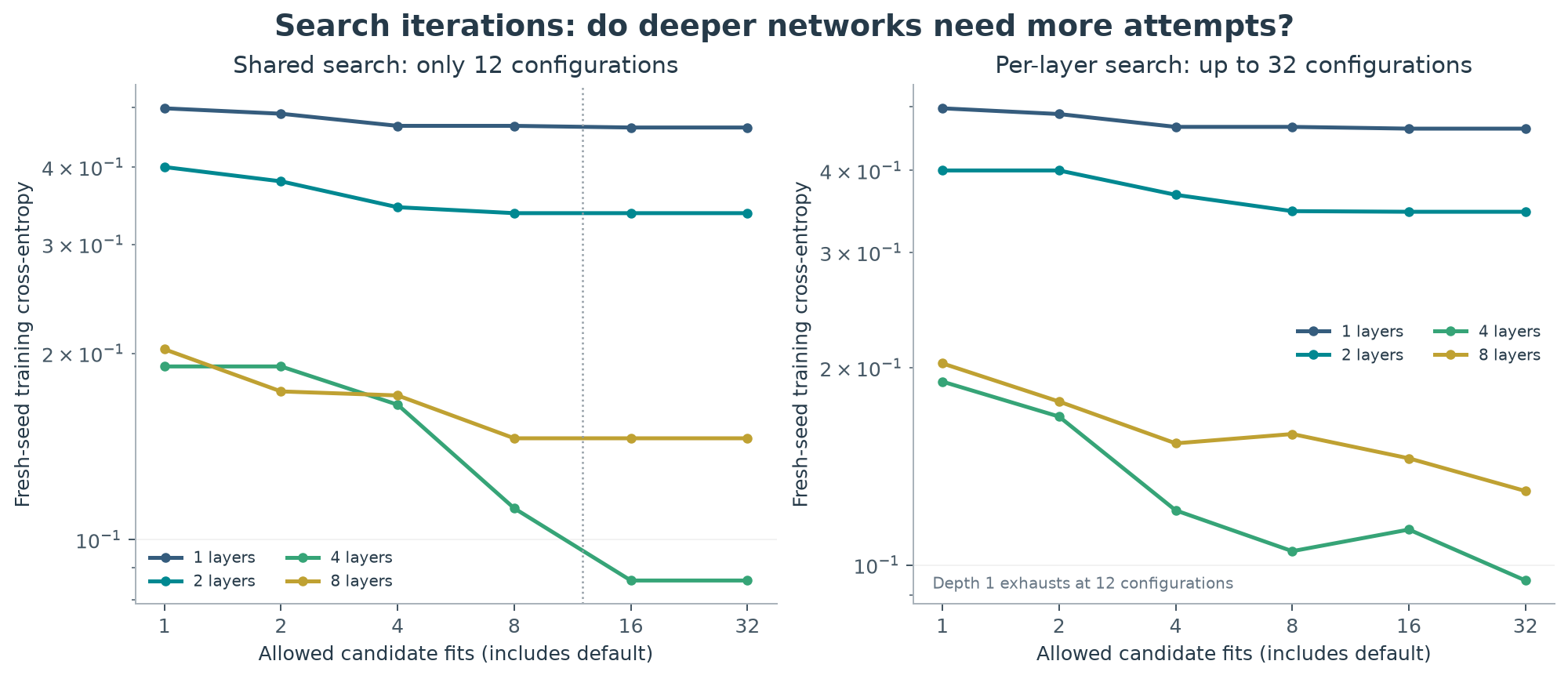
Figure 3 shows how many attempts each depth needs. At depth 1 the per-layer space has only twelve configurations and the curve is nearly flat after four trials. At depth 2 it is flat after about eight. At depths 4 and 8 the curves are still falling at 16 and 32 trials, and the 8-layer curve is noisy because a single early trial can win or lose a repetition. In short, search budgets of 4-8 are enough for shallow networks, while we have not yet seen the deeper searches converge.
Figure 4 puts this on a compute axis. A trial costs more at depth (default fit: 22, 32, 42 and 59 CPU-seconds at 1, 2, 4, 8 layers, under shared machine load), and the per-layer space is far bigger, so 32 trials cost 288, 1,034, 1,470 and 2,052 CPU-seconds. The twelve-configuration shared search cost 288, 388, 557 and 780. On a compute axis the cheap shared search reached the best result at depths 1-4.
Selection on one training seed is optimistic, and the optimism is easy to measure here: the winners' loss on the seed used for selection was lower than their loss after retraining with fresh seeds by about 4%, 15% and 12% at 2, 4 and 8 layers (for example 0.083 versus 0.095 at 4 layers) and was no different at 1 layer. Part of the apparent 4-layer gain (roughly 59% at selection) was selection luck (50% after retraining); a large gain remained.
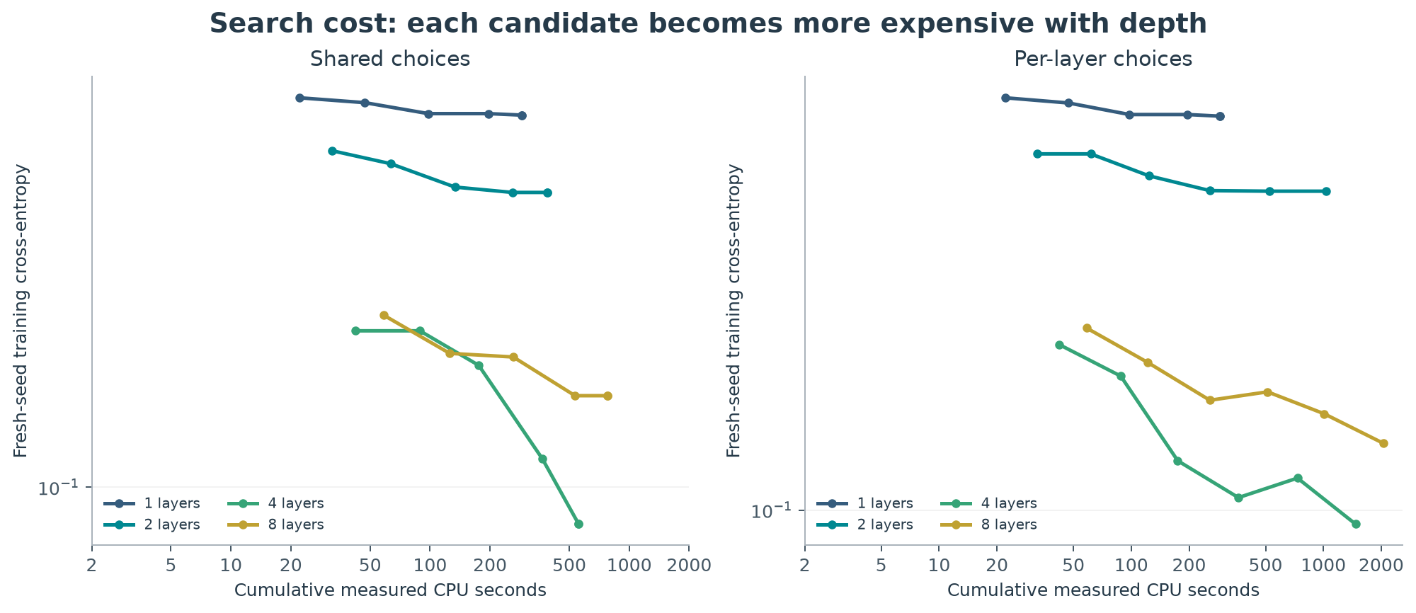
Equal trial counts and equal compute answer different questions. Depth can make each training run more expensive even if it does not increase the number of attempts needed to find a useful architecture. These plots do not estimate an optimal stopping time or the true global optimum. They show the configurations reached by this particular search distribution within the tested allowances.
5What surprised us
1. The default network stalled between 4 and 8 layers, so the fixed 'LeakyReLU + LayerNorm + 3x3' recipe left a lot on the table at depth. Even so, a tuned 8-layer network did not beat a tuned 4-layer one; with plain layers, 16 channels and 20 epochs, extra depth beyond 4 did not pay.
2. One recipe won almost everywhere. GELU + LayerNorm + 5x5 was the best shared recipe in 11 of 12 searches, and the per-layer winners mostly used 5x5 kernels (3-4 of 4 layers at depth 4; 3-6 of 8 at depth 8) with LayerNorm in only 1-5 layers. The search space seems to contain one dominant direction, which is why twelve uniform recipes did about as well as a huge per-layer space.
3. 'Tuning' here also means more parameters. The best recipes use the largest kernel and have about twice the parameters. A parameter-matched comparison could change the interpretation, and is the first thing we would check next.
4. Fitting gains did not become accuracy gains. The deeper networks already overfit, so the architectures chosen for fitting the training set had little effect on test accuracy at 4 and 8 layers (+0.3 and +0.2 points) but did help at 1-2 layers (+1.1 and +1.4 points).
5. Good configurations became more common with depth, not rarer. The fraction of random candidates beating the default was 36%, 57%, 70%, 86%, because the default degraded relative to the space rather than the space degrading.
6. At one layer, the learning rate mattered more than the architecture. Choosing among just three learning rates beat the whole 32-trial architecture search at 1 layer (0.435 versus 0.463) and did nothing at 8 layers, where the architecture search gave a 36% reduction. What limits a network changes with depth.
6Two checks on the explanation
Before the main search we specified controls at depths 1, 4, and 8. First, we keep the default architecture and select among learning rates 0.0003, 0.001, and 0.003 using training loss, then retrain with fresh seeds. Second, we retrain the default and the architectures selected at the 32-trial allowance for 40 epochs. The latter does not repeat architecture search at 40 epochs; it tests the persistence of the 20-epoch selection.
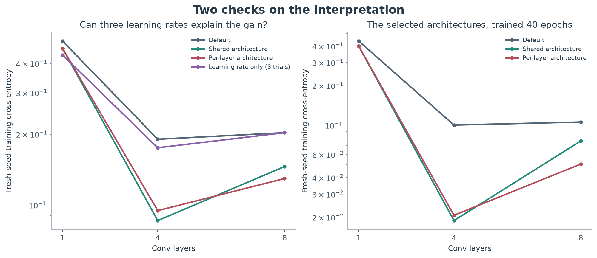
Learning rate only. For the default architecture we chose among learning rates 0.0003, 0.001 and 0.003 by training loss and retrained with fresh seeds. This reduced training loss by 12.7% at 1 layer (0.435; the largest rate was chosen in all three searches), by 8.0% at 4 layers (0.175) and by 0% at 8 layers (0.203; the default rate won every time). So at 1 layer the learning rate alone beat the 32-trial architecture search (0.435 versus 0.463), while at 4 and 8 layers the architecture search gained far more (50% and 36%). The shallow network is limited mainly by how fast it optimizes; the deeper ones by their architecture. This also shows that the growing benefit of architecture tuning is not an artifact of a poor learning rate at depth. The two searches differ in space and budget, so this is a diagnostic and not a matched competition.
Longer training. We retrained the default and the architectures selected at the 32-trial allowance for 40 epochs, without repeating the search. The default improved (training loss 0.436, 0.100 and 0.106 at 1, 4 and 8 layers) but the selected architectures improved more: 0.399, 0.021 and 0.051 for per-layer selections and 0.399, 0.019 and 0.076 for shared selections. Relative to the 40-epoch default that is a reduction of 9%, 79% and 52% (per-layer) and 9%, 81% and 28% (shared). The gains therefore persist, and grow in relative terms, with longer training, so they are not only faster early learning. At 40 epochs the default 8-layer network (0.106) fit about as well as the default 4-layer one (0.100), so part of the 4-to-8-layer stall at 20 epochs was slower optimization, but the tuned 8-layer networks still fit worse than the tuned 4-layer ones (0.051 versus 0.021). Held-out accuracy gains stayed small at depth (+0.4 and +0.2 points at 4 and 8 layers, versus +1.2 at 1 layer).
7What to investigate next
- Match parameter counts: compare tuned and default networks with equal parameters (for example by adjusting channels when kernel size changes) to separate better design from added capacity.
- Run a longer or better-optimized training recipe at 6-8 layers, or add residual connections, to see whether the stall beyond 4 layers is an optimization limit and whether the tuning gain keeps growing with depth.
- Add depths 3 and 6 and more search repetitions (we have three per cell) to turn the growth curve from suggestive into precise, especially at 8 layers where results varied most.
- Test generalization directly: select on validation loss or accuracy and compare, since fitting gains barely carried over to test accuracy at depth.
- Use a smarter search (successive halving, or re-fitting the top candidates with extra seeds) to see whether the bigger search spaces at depth can be searched more cheaply, since the shared recipe got most of the way for about 40% of the cost.
- Repeat on a harder image task (for example CIFAR-10) where depth continues to help, to check that the pattern of larger tuning gains at greater depth is not specific to this small dataset.
- Tune the learning rate and architecture jointly at each depth, since the learning rate alone beat architecture search at 1 layer but not at 4-8 layers.
8Limitations
- One dataset, one fixed training set, three independent searches, and narrow plain CNNs. Bands describe run variation conditional on this split; they are not confidence intervals for a broad population of tasks.
- Depth increases parameter count at fixed width, while the choices of kernel size and LayerNorm also change parameter count (5×5 kernels add substantially). This does not isolate depth at matched parameter or inference-compute budgets.
- A fixed learning rate, initialization rule, and training horizon interact with architecture. The two controls probe only part of this dependence; no architecture-specific optimizer tuning is performed in the main experiment.
- Random search without replacement is the only architecture-search procedure. Bayesian, evolutionary, or structured searches may have different depth–budget relationships.
- The objective is fit to a fixed training set, not generalization: a configuration that fits better may generalize worse, and the secondary test accuracies should not be read as evidence about tuning for generalization. A forced default protects the observed single-seed loss, but seed noise can still select an architecture that performs worse under fresh initialization.
- The study is exploratory. Hypotheses and execution settings were fixed before the main search, but this is not an externally preregistered confirmatory study. A few tested depths and budgets do not identify a power law.
- CPU costs are local measurements and can be affected by background activity. They should not be extrapolated to GPU training or large models. No claim is made about the true best architecture in the full space.
9Relation to earlier work
Random search is a standard baseline, and its effectiveness can depend on how many hyperparameters materially affect performance [1]. Joint architecture and hyperparameter search is an established research area [2]. Our focus is the small controlled interaction among depth, finite search allowance, and shared versus per-layer choices. Work on particular residual-network parameterizations demonstrates depthwise hyperparameter transfer [3]; it cautions against treating retuning costs as a universal consequence of depth, but does not establish transfer of the activation/normalization assignments studied here. Repeated selection on a noisy criterion can overfit it [4], motivating the frozen selections and fresh-seed assessment of the selected configurations. Fashion-MNIST supplies the image classification task [5].
[5] Xiao, H., Rasul, K. & Vollgraf, R. Fashion-MNIST dataset and official distribution.
Appendix: the depth-by-budget map
Reproducibility and accounting
Recorded fits: 416 main-search candidates; 171 fresh-seed assessments; 18 additional learning-rate candidates; 90 control assessments. Numerical failures in the main search: 0. Recorded main-search CPU cost: 318.3 minutes. Recorded CPU cost across main search, fresh assessment, and controls: 596.4 minutes, excluding calibration and warmups. CPU minutes add across workers and are not elapsed clock minutes.
The reproduction script checks unique records, complete evaluation seeds, the absence of test fields in search data, the exact incumbent selected on training loss at every checkpoint, and identical depth-one search spaces. Raw JSONL records, frozen selections, protocol settings, the code, and tidy CSV tables are provided in the download bundle. All figures are supplied as PNG, editable SVG, and vector PDF.
Downloads: measurements.csv · summary.csv · controls.csv · protocol.json · code and raw data (zip)