 Gustav
 Abstract
A flow-matching image model normally gets one forward pass per sampling step. We ask what happens if a small U-Net is given several passes at a fixed noise level, and is allowed to pass something forward: nothing, its previous prediction, or a learned “thought” that is rewarded only through how much it helps the next iteration. On CIFAR-10 at 50% and 75% of the way from noise to image, iterating on the prediction helps a 0.4 M-parameter network by only a few hundredths of a dB, because a single pass is already close to the posterior-mean limit, but in a 0.06 M-parameter network thinking recovers about half of what four times more training does. Rewarded thoughts differ sharply from unrewarded ones: shuffling a rewarded 16-channel thought across images costs 2.4 dB, while an unrewarded one is ignored; a linear probe reads the image class from it with up to 44% accuracy against 32% from the noisy image, and it encodes the model's own uncertainty. When only the final iteration is rewarded, early passes become rough drafts that the thought refines into the answer, and zeroing the thought costs 3.5 to 6.5 dB. Feeding raw predictions back is unstable under long thinking in the tiny network, whereas bounded thoughts reach a fixed point. We also compare a discrete 128-bit thought trained with a straight-through gradient and with REINFORCE.
Key findings
- At one noise level, thinking helps a good network very little (+0.03 dB at 50% noise), because a single pass is already near the theoretical limit. In a network with 9× fewer operations it recovers about half of what 4× more training gives.
- Only rewarded thoughts get used. Shuffling a rewarded 16-channel thought across images costs 2.4 dB; an unrewarded one is ignored.
- Thoughts are not pictures. They are noise-like maps with coarse colour regions that carry the image class (up to 44% by a linear probe vs 32% from the noisy image) and the model's own uncertainty.
- Reward only at the end turns early passes into rough drafts (8 to 16 dB) that the thought refines to the answer, and the thought becomes indispensable.
- Long thinking is stable only for bounded thoughts. Raw prediction feedback collapsed after 8 to 16 iterations in the tiny network.
1Introduction
Image generators such as flow-matching and diffusion models turn random noise into a picture by repeatedly asking a neural network one question: given this half-noisy image, which direction leads towards a clean one?1, 2 The network answers in a single forward pass, and then the sampler moves one small step. That means the network gets exactly one shot of computation per step, however hard the step is.
This paper asks what happens if we give the network more time to think about a single step. Concretely, we freeze the noise level, run the same small network several times in a row on the same noisy image, and let each run see something produced by the previous run. We compare three things that could be passed forward:
- Nothing (the ordinary single pass).
- The previous prediction of the clean image, as in self-conditioning.3
- A learned “thought”: a small extra image-shaped message (1, 4 or 16 channels) that the network writes for its own next iteration, which it is free to fill with anything it finds useful.
The interesting part is the third option. A thought has no ground truth. Nobody tells the network what to write. It can only learn to write something useful if it is rewarded for how well the next iteration does. This raises three questions:
- Q1. Does iterating on its own prediction help, and does it keep helping if we let it think far longer than it was trained to?
- Q2. Does a rewarded thought channel do better than a plain prediction feedback, or than a thought that receives no reward?
- Q3. What do the thoughts actually look like, and do they look different at 50% and at 75% of the way from noise to image?
On “rewarding” a thought
Because our thoughts are continuous numbers inside a differentiable network, we do not need reinforcement learning in the usual sense. We unroll the iterations and let the gradient of the final denoising error flow back through the thoughts (backpropagation through time). That gradient is the reward signal: it tells every thought value how to change so that the next iteration does better, with far less variance than a sampled RL reward. As a control we also train a network whose thought receives no gradient (it stays a random function of the features). To test the real RL case, we additionally train discrete thoughts (a grid of bits) in two ways: with a straight-through gradient, and with REINFORCE, where the reward is literally how much better the following iterations denoise.
2Background
Flow matching trains a network to predict the straight-line velocity from noise to data; sampling integrates that velocity.1, 2 Self-conditioning feeds a diffusion model its own previous estimate of the clean sample and improves sample quality.3 Recurrent depth and weight-tied iterations let a fixed set of weights act as an arbitrarily deep network,4, 5 and recent work trains language models to carry hidden “thoughts” across steps.6, 7 In reinforcement learning, REINFORCE gives a way to train discrete, non-differentiable choices from a reward signal alone,8 while the straight-through estimator pretends the discrete choice was differentiable.9 A useful theoretical anchor is that the best possible predictor of the clean image from a noisy one is the posterior mean, and its error is uncorrelated with anything computable from the input (the orthogonality principle). This both limits how much iteration can help and tells us what a “useful thought” cannot be: it cannot be a copy of the signed error.
3Experimental setup
3.1Flow matching at a fixed noise level
Images are CIFAR-1010 (all 50,000 training images for training, the official 10,000 test images for every number reported), scaled to [−1, 1] with random horizontal flips. A noisy image at time t is xt = t·x1 + (1−t)·z with Gaussian noise z, and the network predicts the velocity v = x1 − z. The clean-image prediction is x̂1 = xt + (1−t)·v̂, and we report its quality as PSNR (higher is better; random-looking noise at t = 0.5 scores 11.1 dB). We call t the static position: t = 0.5 means the image is halfway from pure noise to clean, t = 0.75 means three quarters of the way. A separate model is trained for each static position, so that the “thinking” of that model is about exactly that noise level. We also train general models over all t so that we can actually generate images.
3.2A tiny U-Net that can iterate
The network is a small U-Net with three resolution levels (32, 16 and 8 pixels), group normalisation, SiLU activations and time embedding: 0.4 M parameters, or 0.06 M in the “tiny” version used to test whether thinking can substitute for capacity. One iteration receives the noisy image concatenated with the state passed from the previous iteration (nothing, the previous prediction, or a thought) and returns the velocity plus, for thought models, the next thought (a tanh-bounded map of 1, 4 or 16 channels at full resolution). The first iteration receives zeros.
3.3The variants
| Name | What is passed forward | Training signal |
|---|---|---|
| B1 | nothing (single pass) | standard flow-matching loss |
| B4x | nothing | same, but 4× more training steps (compute-matched to K = 4) |
| Bw | nothing, ~4× wider network | same (matches the inference compute of 4 iterations) |
| PFd | previous prediction | loss at every iteration, no gradient through the fed-back prediction (standard self-conditioning) |
| PFb | previous prediction | same, with gradient flowing through it |
| THr | learned thought, 4 channels | not rewarded: no gradient reaches the thought, so it stays a random function of the features |
| TH1 / TH4 / TH16 | learned thought, 1 / 4 / 16 channels | rewarded: loss at every iteration, gradient through the thought |
| THf | learned thought, 4 channels | rewarded only at the end: the loss is applied to the last iteration only, so intermediate passes are free to be pure computation |
| BITST / BITRL | 2 channels of 8×8 bits | discrete thought, straight-through gradient / REINFORCE |
Models prefixed with t (tB1, tTH4, tTHf, …) are the same designs in the capacity-starved tiny network. All models of a given kind train with the same recipe (AdamW, learning rate 2·10−3 with cosine decay, batch size 128, 2,500 steps unless stated). Compute is matched in two ways: B4x matches the training compute of K = 4 iterating models, and Bw matches their inference compute.
3.4What we measure
- PSNR versus thinking iterations, from 1 to 32, on 5,000 test images with fixed noise (the same noise for every model, so differences are paired). The models were trained with at most K = 4 or 8 iterations, so iterations beyond that test whether thinking extrapolates.
- Interventions on the thought: zero it, shuffle it across images, replace it with the thought computed from the same image under a different noise draw, or add noise. If a thought carries image-specific information that the next pass uses, these should hurt.
- Linear probes from the thought to things we care about: the clean image's low and high spatial frequencies, the noise, the model's own uncertainty (the absolute error), and the image class.
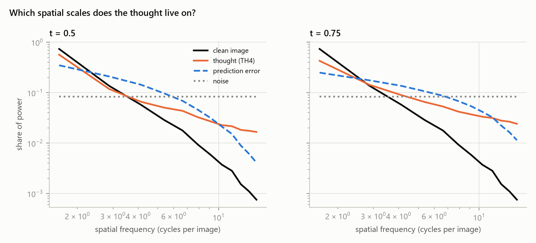
- Power spectra of the thought maps, to see which spatial scales they carry.
- Generation quality for the general models: a Fréchet distance computed in the feature space of a small CIFAR-10 classifier trained for this purpose (not comparable to published FID values).
4Results
4.1Does thinking help? Barely, when the network is already good (Q1)
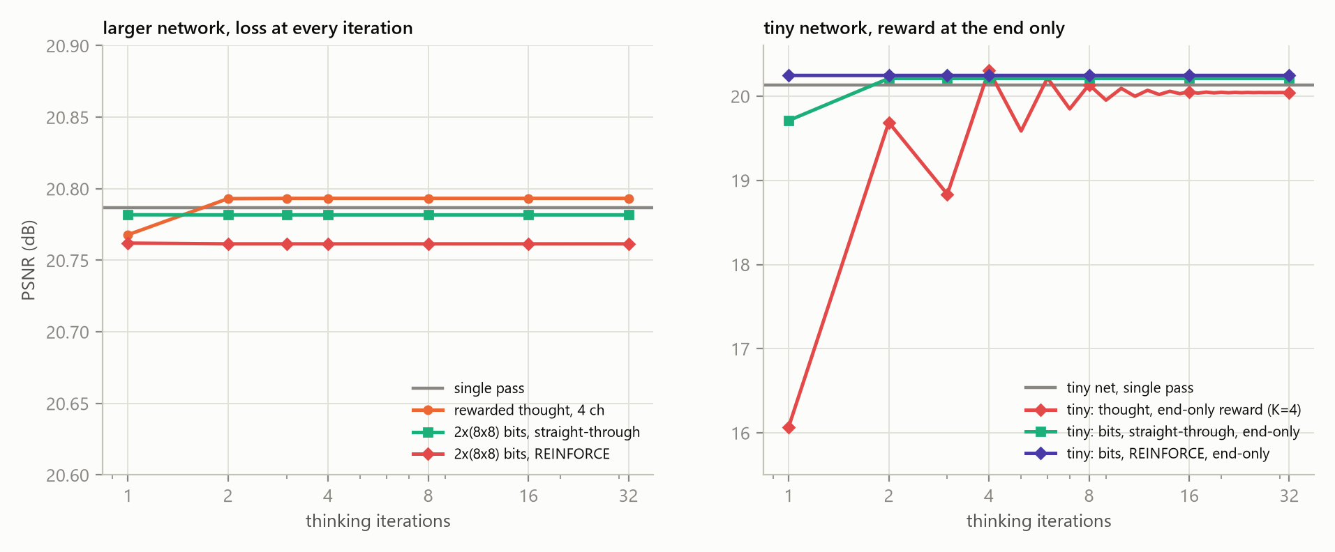
With the 0.4 M-parameter U-Net the answer is: only a little. At t = 0.5 the single-pass model scores 20.79 dB. Feeding its own prediction back (PFd) raises its first-pass 20.75 dB to 20.82 dB after four iterations, which is +0.03 dB relative to the single pass. At t = 0.75 the numbers are 25.94 dB for the single pass and 25.99 dB for PFd (+0.06 dB). Spending the same resources differently does better: training the single-pass model four times longer gives +0.14 dB at t = 0.5, and a four-times-wider single-pass model gives +0.11 dB (t = 0.5) and +0.21 dB (t = 0.75). To check how much of this is training noise, we trained a second seed of five of the models: the single-pass model changed by −0.01 dB, the fed-back-prediction model by −0.00 dB and the rewarded 4-channel thought by −0.00 dB between seeds, so differences of a few hundredths of a dB should not be over-read.
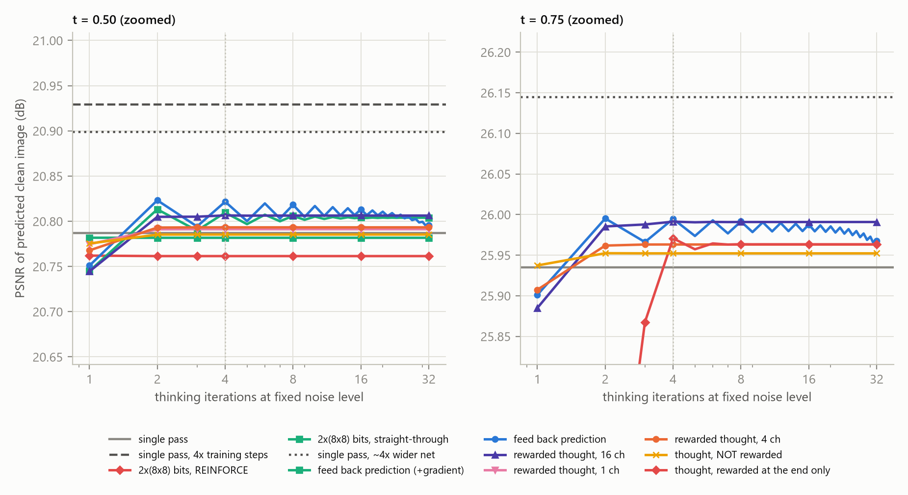
This is what theory predicts. At a fixed noise level the best possible predictor is the posterior mean of the clean image given the noisy one, and the plain network is already close to it: even a four-times-wider network gains only about 0.1 dB at t = 0.5. Thinking can approach that limit but cannot pass it, so a network that is close to the limit has almost nothing to gain.
4.2When capacity is scarce, thinking buys a real fraction of it
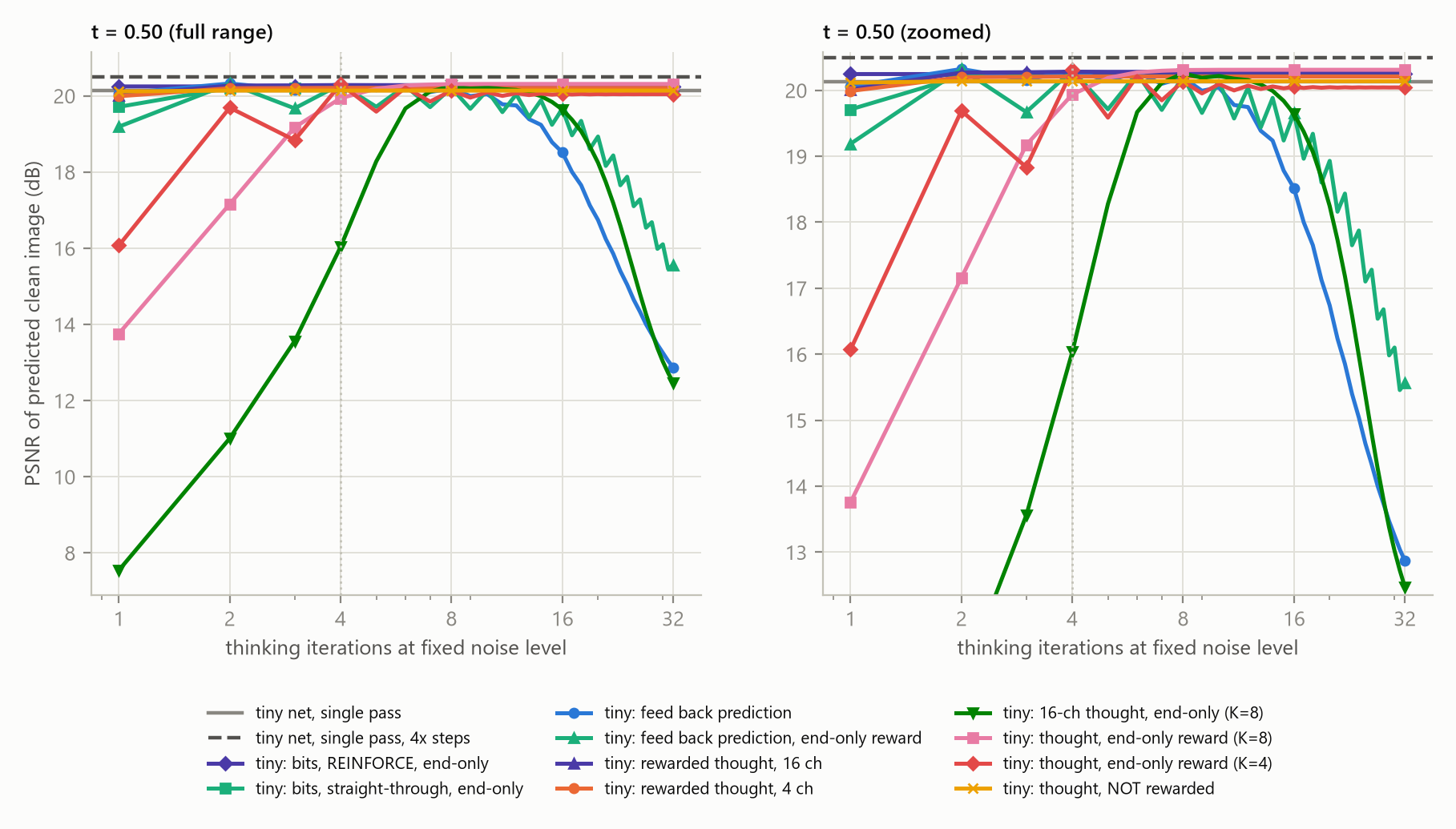
To give thinking something to fix, we repeated the experiment with a capacity-starved network of 0.06 M parameters (about 9× fewer multiply-adds per pass). Its single pass scores 20.13 dB and training it four times longer reaches 20.50 dB, so there is a gap of 0.37 dB to close. Thinking with four iterations reaches 20.32 dB (fed-back prediction), 20.31 dB (thought, rewarded at the end) and 20.28 dB (rewarded 16-channel thought), i.e. about 53% of the gap that four times more training closes, at four times the inference cost but with no extra training data or steps beyond the unrolling. The tiny network is noisier between training runs than the larger one: a second seed changed the single pass by −0.07 dB, the end-rewarded thought by −0.08 dB and the rewarded 4-channel thought by +0.02 dB, so the "about half" should be read as roughly 40 to 60%.Different ways of passing information forward end at nearly the same level, which suggests that what limits the tiny network is how much computation it can do on this noise level, not what kind of message it sends.
How long can it think?
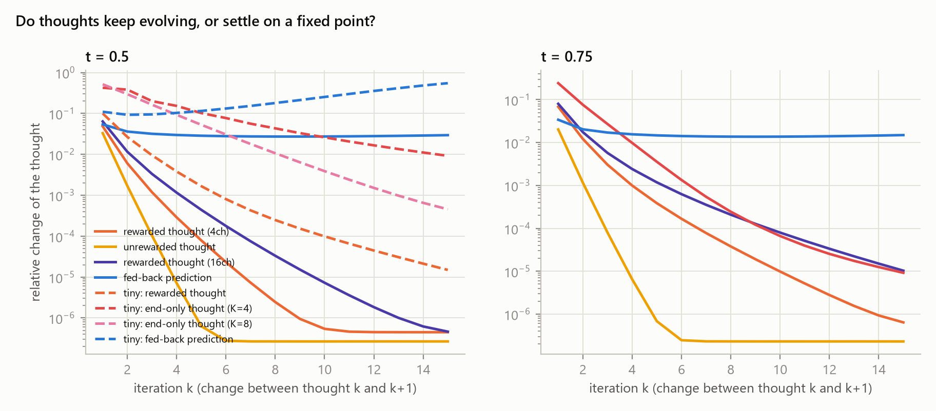
Letting the models think far longer than they were trained to (up to 32 iterations) gives two different behaviours. Thoughts that are bounded (tanh) and trained for enough iterations settle on a fixed point and stay there: the 4-channel end-rewarded thought trained with 8 iterations holds 20.31 dB at iteration 32. Feeding the raw prediction back is unstable in the tiny network: its quality peaks after two iterations (20.32 dB) and falls to 12.9 dB by iteration 32, because small errors in the prediction are amplified each time it is fed back. The 16-channel end-rewarded thought, which has the most freedom, also drifts out of the region it was trained on (12.5 dB at iteration 32). Longer training horizons help: the same design trained for 4 iterations (tTHf) slides gently to 20.04 dB at 32, while training for 8 iterations (tTHf8) does not slide at all.
4.3Is the reward what makes a thought useful? (Q2)
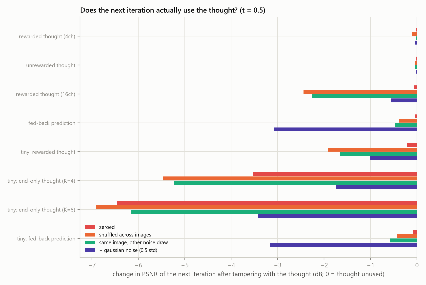
Yes for what the thought contains, much less for the final accuracy. The cleanest test is the thought that receives no gradient (THr, tTHr): it stays a random function of the features. It scores the same as the single pass (t = 0.5: 20.79 dB against 20.79 dB), and the next iteration ignores it: shuffling it across images changes the next prediction by −0.04 dB. A rewarded 16-channel thought is used in an image-specific way: shuffling it across images costs 2.4 dB at t = 0.5 and 2.6 dB at t = 0.75, and giving the network the thought from the same image with different noise costs 2.3 dB, so the thought encodes noise-specific information rather than only the image identity. In the tiny network a rewarded thought gains +0.07 dB (4 channels) and +0.14 dB (16 channels) over the unrewarded one. The 4-channel thought of the larger network, in contrast, is hardly used at all (−0.11 dB when shuffled): with a loss at every iteration, the first pass is already pushed to be as good as it can be, so the network has little reason to rely on a message from itself.
4.4Reward only at the end: genuine multi-step thinking
When the loss is applied only to the last iteration (the “end-only” models), the first passes are free to be rough drafts, and they are: the tiny network's first pass scores 16.1 dB (K = 4) or 13.8 dB (K = 8), and quality climbs steadily to about 20.3 dB by the last iteration. Here the thought is indispensable: zeroing it costs 3.5 dB (K = 4) and 6.5 dB (K = 8), against 0.2 dB for the deep-supervised thought. The same pattern appears in the larger network at t = 0.75, where the first pass of the end-only thought scores 22.4 dB and the fourth 25.97 dB. This is the closest our toy gets to “thinking” in the sense of using several steps of private computation to reach an answer, and its final accuracy is not better than that of deep supervision: it is the process that differs, not the result.
4.5What do the thoughts look like, and does it differ between 50% and 75%? (Q3)
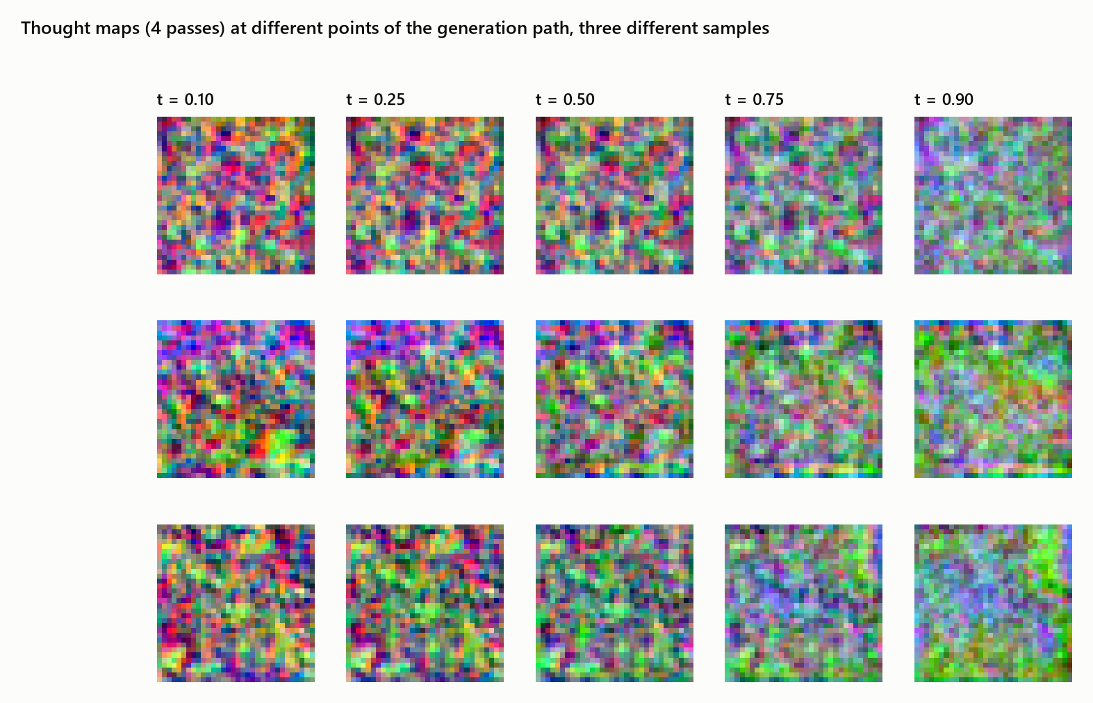
Figures 5 and 6 show the 16-channel rewarded thought as a colour image (first three principal components of its channels) next to the clean-image prediction. Three things stand out.
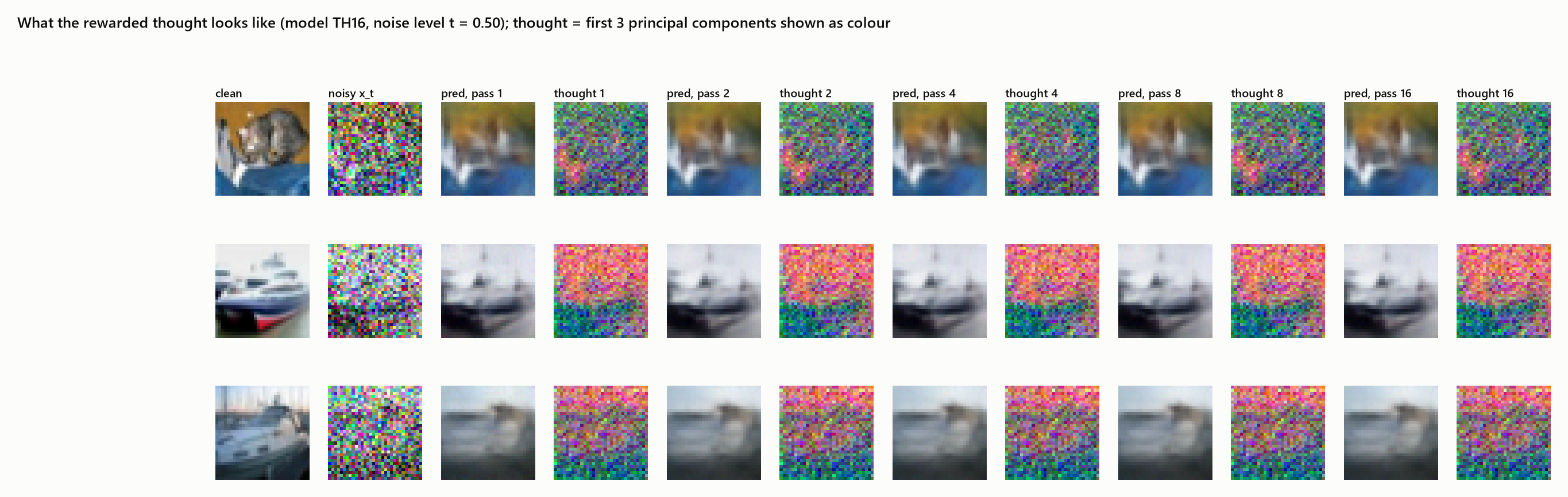
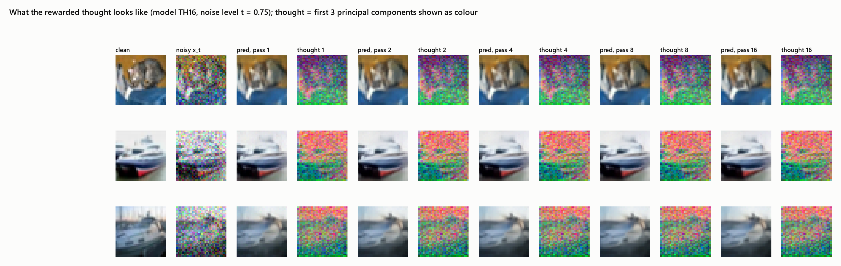
- Thoughts are not pictures of the answer. They look like textured, noise-like maps with large-scale colour regions that follow the layout of the object (a horizon, a hull, the outline of an animal), rather than like a cleaner version of the image. The 4-channel deep-supervised thought is dominated by low spatial frequencies: 57% of its power sits in the lowest frequency band, against 73% for the clean image.
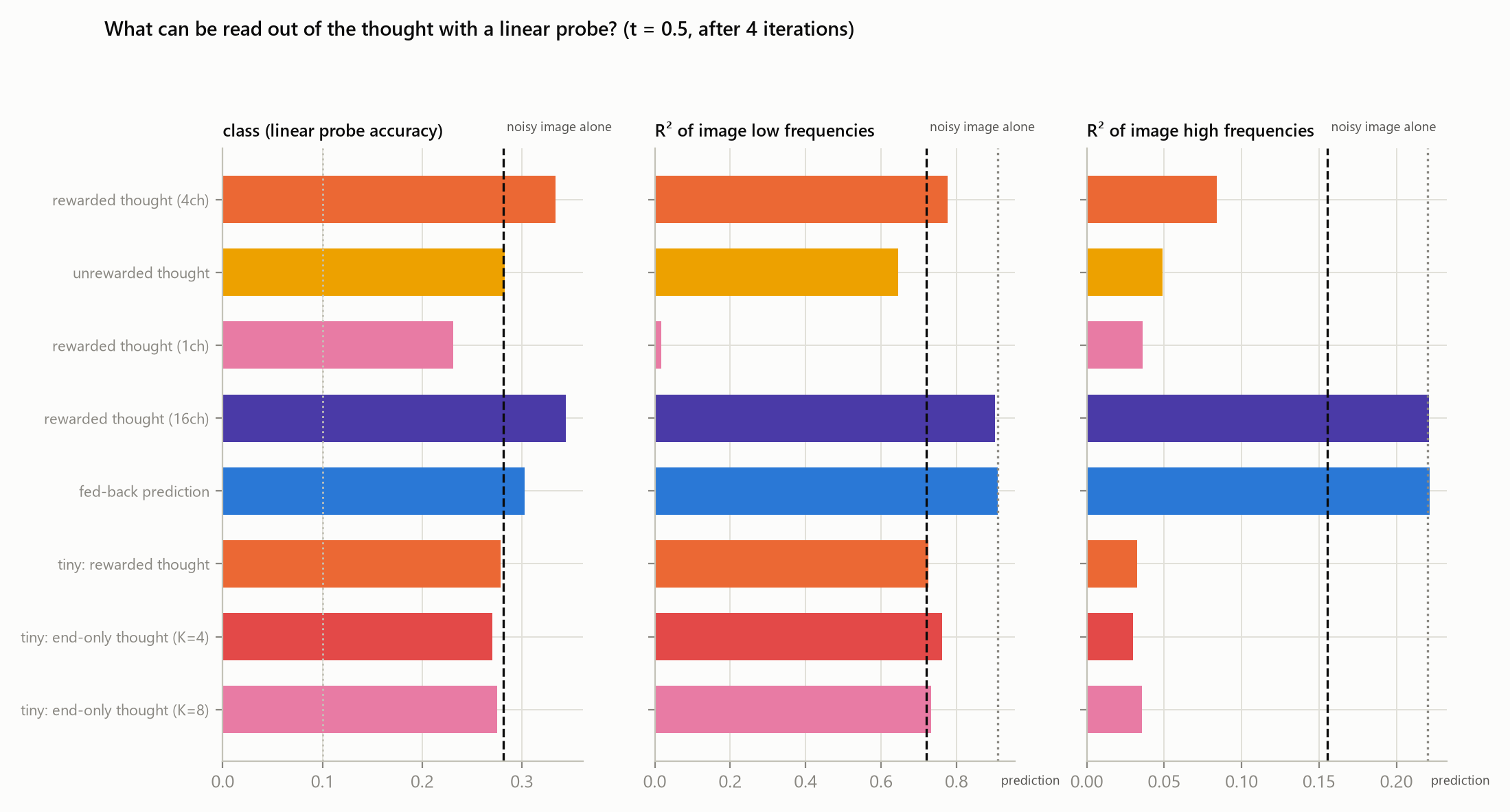
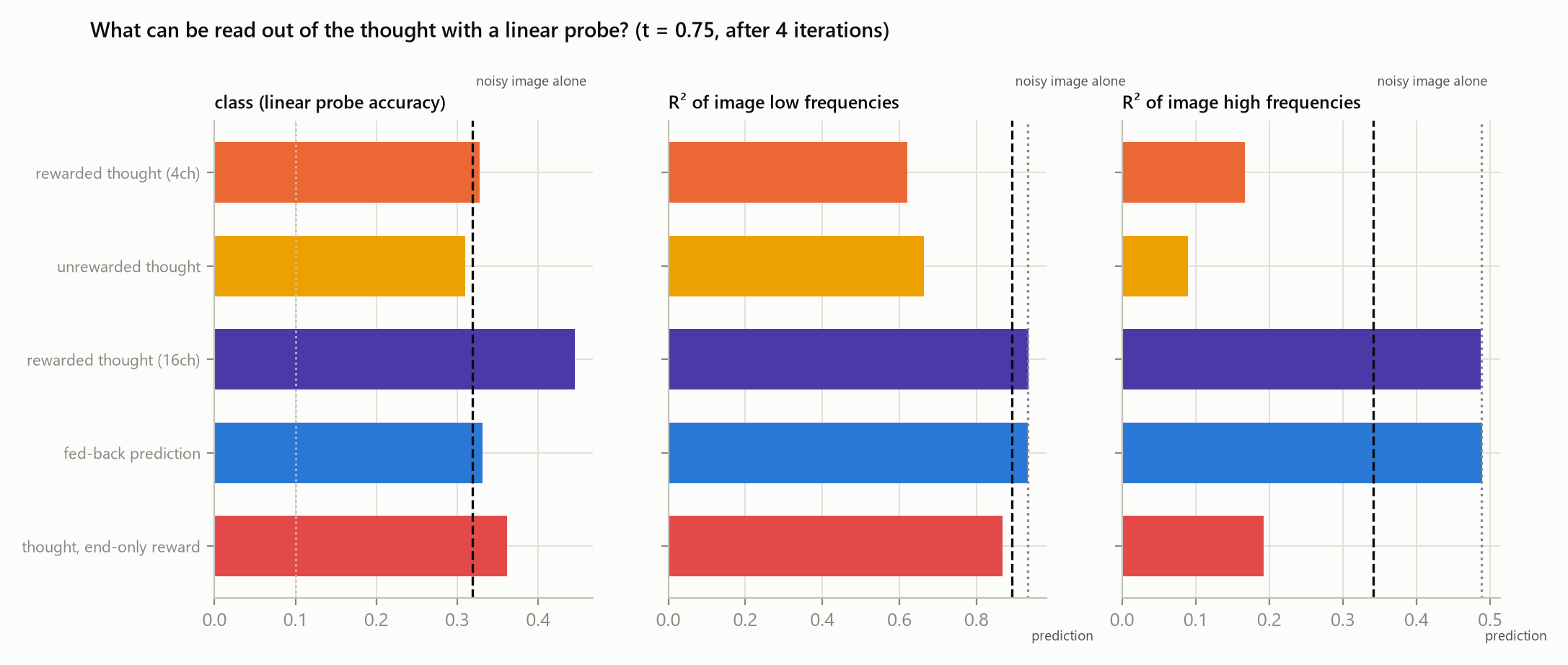
- What is in them depends on how much room they have. A linear probe (Figure 7) shows that the 16-channel rewarded thought re-encodes the image prediction almost completely (R² for low frequencies 0.90 at t = 0.5 and 0.93 at t = 0.75, equal to the prediction itself), whereas the 4-channel thought keeps mostly the coarse layout (0.78) and the 1-channel thought holds almost nothing a linear probe can find (0.02). At t = 0.75 it also carries the high-frequency detail (0.49); at t = 0.5, where the details are mostly buried in noise, it carries far less (0.22), which is the main visible difference between the two static positions.
- They carry semantic information and the model's own uncertainty. From the 16-channel thought a linear classifier recovers the image class with 44% accuracy at t = 0.75 (34% at t = 0.5), compared with 32% from the noisy image and 32% from the clean-image prediction (chance is 10%). The unrewarded thought manages 31%. The thought also helps predict how wrong the prediction is: the share of variance of the absolute error that a probe explains rises from 0.012 (noisy image and prediction) to 0.118 when the thought is added (t = 0.75), a confidence signal that exists in no other channel. The signed error, by contrast, cannot be predicted from anything, as the orthogonality principle requires.
4.6Discrete thoughts: backpropagation versus real reinforcement learning
To test the reinforcement-learning version of the idea, we replaced the continuous thought with a grid of bits (2 channels of 8×8 = 128 bits per image) that is sampled and passed forward. The network is trained in two ways: straight-through (BITST), where gradients pass through the sampling as if it were a smooth function, and REINFORCE (BITRL), where the bits are sampled, and the policy is improved with the reward given by how much better the following iterations denoise (advantage = discounted future loss relative to the batch average). In the larger network, with a loss at every iteration, neither discrete thought was used: both stayed at the single-pass level (20.78 dB straight-through, 20.76 dB REINFORCE, against 20.79 dB), and the sampling probabilities stayed at their maximum entropy, i.e. the bits remained coin flips. That is the same story as for the continuous 4-channel thought: nothing forces the network to rely on a message from itself. In the tiny network, rewarded at the end only, the two methods split. With a straight-through gradient the 128 bits became decisive (their sampling entropy fell to about half of its maximum) and were used: the first pass scores 19.71 dB, the second and later passes 20.21 dB, which equals the continuous 4-channel thought of the same network (20.21 dB). So a 128-bit message is enough to carry what the network needed. With REINFORCE the network ended in a different solution: its sampling entropy stayed at the maximum (the bits remained coin flips) and it learned to ignore them entirely (the score is 20.25 dB on every iteration), so the bits never became useful. The reward is a single noisy number per image shared by all 128 bits, and the network had no use for the bits yet when the policy started to learn, so there may have been no signal to find: a plausible reading is the classic chicken-and-egg problem of learning a communication channel by reinforcement (we did not test this explanation directly). A gradient through the message, where one exists, is the far better teacher; REINFORCE is the fallback for truly discrete or non-differentiable messages and would need longer training, a better baseline or a warm start to compete here.
4.7Does thinking help real generation?
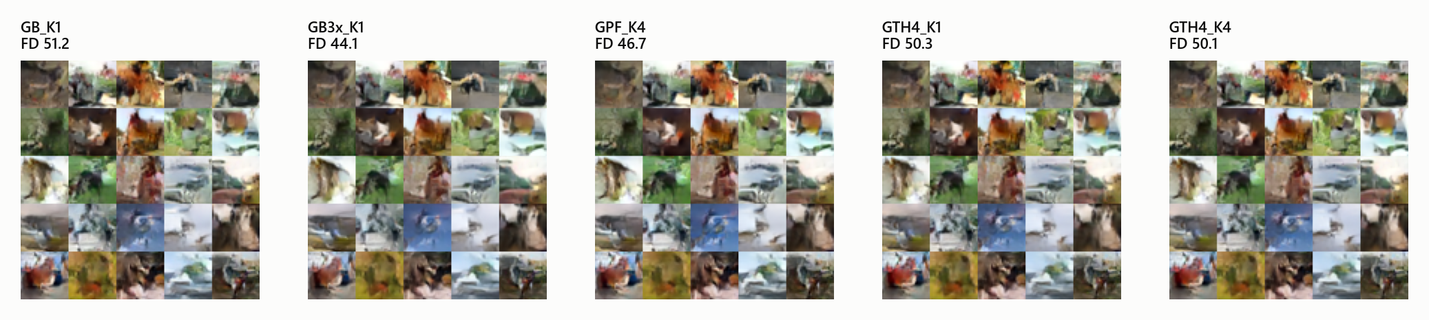
The static-position models cannot generate images, so we trained three models on all noise levels (the single-pass model GB, and variants with a fed-back prediction GPF and a rewarded 4-channel thought GTH4, each unrolled for 3 iterations in training, 5,000 steps) plus a single-pass model trained three times longer. Images are generated with 20 Euler steps of the flow, and at each step the model thinks for K iterations at the current noise level before the step is taken. We score 5,000 samples by the Fréchet distance (FD) between their features and those of real test images in a small classifier trained for this paper; two sets of real images differ by 0.39 on this scale. Lower is better.
| Model and thinking per step | FD (lower is better) |
|---|---|
| single pass (GB) | 51.23 |
| single pass, 3x training (GB3x) | 44.12 |
| fed-back prediction, K=1 (GPF) | 52.00 |
| fed-back prediction, K=2 | 47.81 |
| fed-back prediction, K=4 | 46.72 |
| fed-back prediction, K=8 | 46.61 |
| fed-back prediction, K=2, state carried across steps | 50.44 |
| fed-back prediction, K=4, state carried | 52.92 |
| fed-back prediction, K=8, state carried | 53.44 |
| thought (GTH4), K=1 | 50.33 |
| thought, K=2 | 50.50 |
| thought, K=4 | 50.09 |
| thought, K=8 | 50.06 |
| thought, K=2, state carried across steps | 50.77 |
| thought, K=4, state carried | 50.10 |
| thought, K=8, state carried | 50.06 |
The best configuration here is single pass, 3x training (GB3x) with FD 44.12, against 51.23 for the single pass and 44.12 for the single pass trained three times longer.
5What surprised us
1. Thinking barely helps a network that is already good
At 50% noise, feeding the prediction back for four iterations gained +0.03 dB over a single pass, while simply training four times longer gained +0.14 dB. A single forward pass of a small U-Net is already close to the theoretical limit for one noise level.
2. A message nobody specified ends up carrying meaning
The 16-channel thought was never told to encode anything, yet a linear classifier reads the image class from it with 44% accuracy at t = 0.75, against 32% from the noisy image and 32% from the model's own clean-image prediction.
3. A thought is only used if it is rewarded, and deep supervision removes the need for it
The thought that received no gradient was ignored (shuffling it changed the next prediction by -0.04 dB). The rewarded 16-channel thought mattered (-2.4 dB when shuffled). With a loss at every iteration, the 4-channel thought froze after one pass and was barely used; only when we rewarded the final iteration alone did thoughts become indispensable (zeroing them cost 3.5 to 6.5 dB).
4. Feeding the prediction back is unstable under long thinking in a tiny network
The tiny fed-back-prediction model peaks after two iterations (20.32 dB) and has fallen to 12.9 dB by iteration 32. Bounded thoughts that were trained long enough stayed at their level indefinitely.
5. The thought contains a confidence signal that no other channel has
Adding the 16-channel thought to the noisy image and the prediction raises the share of the absolute prediction error that a linear probe explains from 0.012 to 0.118 at t = 0.75: the network writes down how unsure it is.
6. The gradient beat reinforcement learning, as it should, but RL still learned something useful
In the larger network, with a loss at every iteration, neither discrete thought was used: both stayed at the single-pass level (20.78 dB straight-through, 20.76 dB REINFORCE, against 20.79 dB), and the sampling probabilities stayed at their maximum entropy, i.e. the bits remained coin flips. That is the same story as for the continuous 4-channel thought: nothing forces the network to rely on a message from itself. In the tiny network, rewarded at the end only, the two methods split. With a straight-through gradient the 128 bits became decisive (their sampling entropy fell to about half of its maximum) and were used: the first pass scores 19.71 dB, the second and later passes 20.21 dB, which equals the continuous 4-channel thought of the same network (20.21 dB). So a 128-bit message is enough to carry what the network needed. With REINFORCE the network ended in a different solution: its sampling entropy stayed at the maximum (the bits remained coin flips) and it learned to ignore them entirely (the score is 20.25 dB on every iteration), so the bits never became useful. The reward is a single noisy number per image shared by all 128 bits, and the network had no use for the bits yet when the policy started to learn, so there may have been no signal to find: a plausible reading is the classic chicken-and-egg problem of learning a communication channel by reinforcement (we did not test this explanation directly). A gradient through the message, where one exists, is the far better teacher; REINFORCE is the fallback for truly discrete or non-differentiable messages and would need longer training, a better baseline or a warm start to compete here.
6Limitations
- One dataset, one tiny architecture family, short training. All models are tiny U-Nets trained for 2,500 steps; conclusions about larger models may differ.
- Static noise levels. Most results are for a model trained at one noise level. The general models connect them to real sampling, but we did not explore carrying thoughts across sampling steps in depth.
- Small effects. Many differences between variants are a few hundredths of a dB. We trained a second seed of some models to gauge training noise, but the number of seeds is small.
- The generation metric is not FID. It is a Fréchet distance in the features of a small classifier trained on CIFAR-10, with 5,000 samples, and is meaningful only relative to the other numbers in this paper.
- Probes are linear and the thought maps are only a few channels. Absence of a linear signal is not absence of information.
- Discrete RL variant is lightly tuned. REINFORCE has high variance and we did not sweep its hyper-parameters.
7Frequently asked questions
Does letting a diffusion or flow model think longer improve its images?
In our tiny CIFAR-10 experiments the effect at a single noise level was small for a network that was already good (a few hundredths of a dB) but substantial for a capacity-starved one, where four thinking iterations recovered about half of the gain from four times more training.
What is a latent thought in a denoiser?
A small extra feature map the network writes after each pass and reads in the next. It has no target; it is trained only through its effect on later predictions.
Do you need reinforcement learning to reward a thought?
Not if the thought is continuous: backpropagating through the iterations gives a low-variance reward signal. Reinforcement learning (REINFORCE) is needed only for discrete thoughts, and we compare the two.
What do the thoughts look like?
Noise-like maps with large-scale colour regions that follow the object layout, not cleaner images. A 16-channel thought re-encodes the prediction and also carries the image class and the model's own uncertainty.
Is it stable to let the model think for a very long time?
Only for bounded, well-trained thoughts. Feeding the raw prediction back drifted and collapsed in the tiny network after about 8 to 16 iterations.
Statement on AI assistance
The experiments were designed, run and written up by the author together with Claude (Anthropic), an AI assistant, which wrote the code and the first draft of the text. The numbers come from the runs described; the author is responsible for the content.
References
- Lipman, Y., Chen, R. T. Q., Ben-Hamu, H., Nickel, M., Le, M. (2023). Flow Matching for Generative Modeling. ICLR. arXiv:2210.02747
- Liu, X., Gong, C., Liu, Q. (2023). Flow Straight and Fast: Learning to Generate and Transfer Data with Rectified Flow. ICLR. arXiv:2209.03003
- Chen, T., Zhang, R., Hinton, G. (2023). Analog Bits: Generating Discrete Data using Diffusion Models with Self-Conditioning. ICLR. arXiv:2208.04202
- Dehghani, M., Gouws, S., Vinyals, O., Uszkoreit, J., Kaiser, Ł. (2019). Universal Transformers. ICLR. arXiv:1807.03819
- Graves, A. (2016). Adaptive Computation Time for Recurrent Neural Networks. arXiv:1603.08983
- Hao, S., Sukhbaatar, S., Su, D., Li, X., Hu, Z., Weston, J., Tian, Y. (2024). Training Large Language Models to Reason in a Continuous Latent Space. arXiv:2412.06769
- Geiping, J., McLeish, S., Jain, N., Kirchenbauer, J., Singh, S., Bartoldson, B. R., Kailkhura, B., Bhatele, A., Goldstein, T. (2025). Scaling up Test-Time Compute with Latent Reasoning: A Recurrent Depth Approach. NeurIPS. arXiv:2502.05171
- Williams, R. J. (1992). Simple statistical gradient-following algorithms for connectionist reinforcement learning. Machine Learning 8, 229-256.
- Bengio, Y., Léonard, N., Courville, A. (2013). Estimating or Propagating Gradients Through Stochastic Neurons for Conditional Computation. arXiv:1308.3432
- Krizhevsky, A. (2009). Learning Multiple Layers of Features from Tiny Images. Technical report, University of Toronto. CIFAR-10 page