Do Good Small Blocks Make Good Deep Networks? Block-Level Architecture Search, Pretrained Stacking and Depth-vs-Width Scaling on Low-Data CIFAR-10

Abstract

Neural architecture search often finds a small building block and stacks copies of it into a deep network, assuming that (i) a block that is good alone stays good when stacked, and (ii) pretraining the block gives a better starting point than random initialisation. We test both on CIFAR-10 with 5,000 labelled training images, using 48 random blocks, stacks of 1, 2, 4 and 8 blocks, two seeds per configuration, and compute-matched controls. Block rankings from 1-block classifiers agreed with 2-block rankings (Spearman 0.73) but not with 4- or 8-block rankings (0.06 and -0.08); the best 1-block design ranked 17th of 48 at 8 blocks. The main cause was trainability: plain blocks collapsed when stacked while residual blocks kept improving. Pretraining on the same data gave much faster early convergence and +2 to +3.5 points over random initialisation at 4 and 8 blocks, but a random-initialised network trained for the same total compute recovered much of that gain; transferring a block without its stem gave no benefit. At equal compute, evaluating candidates at the deployment depth beat searching with 1-block proxies. Widening beat stacking at matched cost for the selected block, and pretraining gains did not shrink with more labelled data. Limitations: one dataset, few seeds (2 to 4), and searches simulated by resampling trained pools.

1Introduction

Most neural architecture search (NAS) methods look for a good whole network, or for a small repeated cell that is later stacked into a whole network.^{1, 2, 3, 4} The cell-based idea is attractive because searching a small thing is cheap: find a good building block on a small problem, then build something big out of copies of it.

That idea rests on two assumptions that are easy to state and surprisingly rarely tested in isolation:

1. Architecture transfer. A block that is good by itself stays good when it is repeated many times inside a deeper network.
2. Weight transfer. If we also train the small block first and copy its learned weights into the deeper network, the deeper network trains faster or ends up better than one initialised at random.

This paper tests both assumptions in the smallest setting where they can be tested carefully: CIFAR-10 images,⁵ a deliberately small labelled training set (5,000 images), a space of 48 randomly sampled blocks, and enough repeated runs (seeds) to put error bars on every claim. Everything runs on a single consumer GPU (GTX 1070), and every number in this paper comes from runs we actually performed.

We ask five concrete questions:

• Q1. Does the ranking of blocks as 1-block classifiers predict their ranking when stacked 2, 4 and 8 times? (architecture transfer)
• Q2. Does initialising a stack with pretrained blocks beat random initialisation, once total compute is matched? (weight transfer)
• Q3. Is pretraining more valuable for an optimised block than for a random one, and does it depend on how much labelled data there is?
• Q4. At equal search compute, is it better to search for a small block and stack it, or to search directly over deeper networks, or to just take a random block?
• Q5. Given a good block, is it better to scale it by stacking (depth) or by widening it?

2Background and related work

Searching for cells and stacking them

NASNet searched for a convolutional cell on CIFAR-10 and then stacked copies of it to build networks for ImageNet.¹ Evolution-based² and gradient-based³ searches followed the same recipe. The recipe works in practice, but benchmarks of NAS repeatedly found that random search is a strong baseline⁶ and that carefully-tuned random policies are hard to beat,^{7, 8} which makes the question "how much does the search itself contribute?" a live one. Tabular benchmarks such as NAS-Bench-101 and NAS-Bench-201 made it possible to measure how well cheap proxies rank architectures.^{9, 10} Training-free proxies push this further.¹¹ Our Experiment 1 asks the same proxy question for a specific, common proxy: the same block, but shallower.

Pretraining and weight transfer

Greedy layer-wise training was the original way to make deep networks trainable,¹² and later work asked why such pretraining helps.¹³ Feature transferability decreases as layers become more specialised to the source task.¹⁴ Layer-wise supervised training can scale surprisingly far,¹⁵ and function-preserving growth operators allow a shallow network to initialise a deeper one.¹⁶ In language models, stacking a trained shallow transformer on itself to initialise a deeper one speeds up pretraining,^{17, 18} which is the closest precedent for our "copy the pretrained block into every position" variant. In the opposite direction, warm-starting from a model trained on the same data can hurt generalisation compared with a fresh start.¹⁹ Our setting, where the pretraining data is the same few thousand images used for fine-tuning, makes that last concern especially relevant.

Depth versus width

Wide residual networks showed that widening can beat deepening at matched cost,²⁰ while compound scaling argues that depth, width and resolution should be scaled together.²¹ Residual connections²² are central to why depth works at all; without them, gradients decorrelate and very deep plain networks train poorly,²³ which turns out to matter a great deal for our results.

Where this study fits

Rather than proposing a new method, we run a controlled, fully reported experiment that separates architecture transfer from weight transfer, includes compute-matched controls for pretraining, and reports the cases where the intuitive story fails.

3Hypotheses and predictions made in advance

The experiment was planned before any run was made. The hypotheses and the predicted outcomes below were written down first; the table in Section 6 compares them with what we found.

Table 1. Hypotheses and pre-registered expectations.

Hypothesis	Statement	Expected
H1a	Pretrained blocks converge faster than randomly initialised ones.	Moderate confidence yes
H1b	Pretrained blocks reach higher final test accuracy.	Uncertain; scratch training may catch up
H1c	The pretraining advantage changes with the number of stacked blocks.	Uncertain
H1d	Copying the same pretrained block into every position helps.	Low confidence (deeper layers see different feature distributions)
H2a	Optimised blocks beat randomly selected blocks at equal parameter count.	Moderate confidence yes
H2b	The ranking of small blocks predicts the ranking after stacking.	Uncertain
H2c	Small-block search is more compute-efficient than direct full-network search.	Moderate confidence yes
H3	Pretraining helps optimised blocks more than random blocks (interaction).	Open

We also listed in advance which outcomes would count as surprises: random initialisation beating pretraining; the best small block becoming one of the worst large networks; a mediocre small block scaling exceptionally well; random architecture search beating optimised-block search; pretraining only helping with very small datasets; and width scaling consistently beating depth stacking.

4Experimental design

4.1Data and splits

All experiments use CIFAR-10.⁵ From the 50,000 official training images we draw, once and with a fixed seed, class-balanced subsets: a training set of 5,000 images (500 per class), a disjoint validation set of 5,000 used only to select architectures, and a further disjoint 5,000-image "extra" set that is used only in the experiment that asks whether pretraining on additional data helps. The official 10,000-image test set is touched only to report final numbers; no selection ever uses it. Inputs are normalised per channel; training augmentation is a random 4-pixel-padded crop plus horizontal flip.

4.2Networks and the block search space

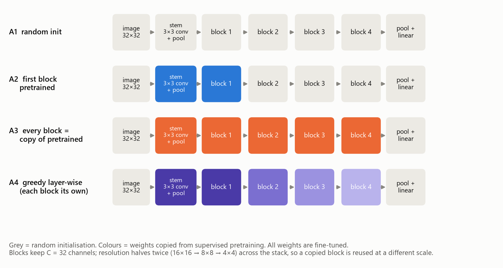
Every network has the same skeleton (Figure 1): a 3×3 convolution stem (32 channels, BatchNorm,²⁴ ReLU) followed by a 2×2 max-pool, then N shape-preserving blocks (N = 1, 2, 4 or 8), then global average pooling and a linear classifier. Blocks are grouped into three resolution stages (16×16, 8×8, 4×4) with a max-pool between stages, so a block copied into a deeper position sees a different spatial scale from the one it was trained on. All blocks have 32 external channels unless stated otherwise (Experiment 5 widens them).

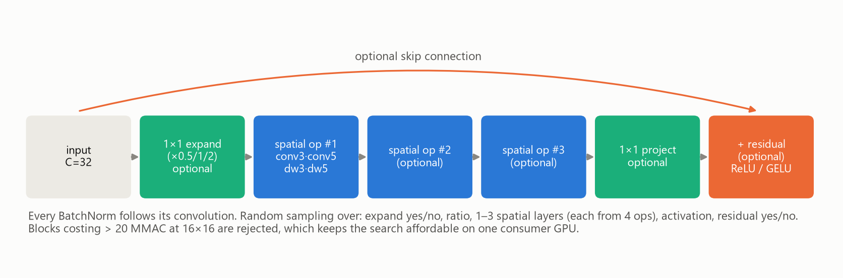
A block is drawn at random from the space in Figure 2: an optional 1×1 expansion (ratio 0.5, 1 or 2) and matching 1×1 projection, one to three spatial layers (each a 3×3 or 5×5 convolution or a depthwise-separable convolution^{25, 26}), ReLU or GELU activation, and an optional residual connection. Blocks costing more than 20 million multiply-accumulates (MACs) at 16×16 are rejected so that the experiments stay affordable. We sampled 48 distinct blocks once and used the same 48 for all experiments.

4.3Training recipe

Every network, whether trained from scratch or fine-tuned, uses the same recipe: SGD with Nesterov momentum 0.9, batch size 128, peak learning rate 0.1 with a 78-step linear warm-up followed by a cosine decay to zero,²⁷ weight decay 5·10⁻⁴ on weights (not on BatchNorm or biases), no label smoothing, fp32. The standard budget is 30 epochs (1,170 steps). Learning rate and epoch count were calibrated once on one block using validation accuracy only (learning rates 0.03, 0.1, 0.2 at 30 and 60 epochs; 0.1 and 0.2 were similar and better than 0.03). A seed controls the random head initialisation, mini-batch order and augmentation; runs in different groups that share a seed share their data order, so comparisons between groups are paired by seed.

4.4Pretraining variants

The block is pretrained as part of a one-block classifier (stem, one block, head) on the 5,000 training images for 30 epochs, then the classification head is discarded. For a stack with N blocks we compare:

• A1: random initialisation.
• A2: stem and the first block initialised from the pretrained one-block network; blocks 2…N random. A2n transfers the block but not the stem (a block taken from a net whose stem it was trained with is partly mismatched if the stem is random).
• A3: stem and every block initialised with a copy of the pretrained block (each copy has its own BatchNorm parameters and statistics).
• A4: independent greedy layer-wise supervised pretraining: block k is trained at the resolution it will have in the final network, on top of the frozen pretrained blocks 1…k−1 and a fresh head, for 20 epochs per stage.
• A2d / A3d: as A2 / A3 but the block was pretrained on the disjoint extra 5,000 images, so that any gain cannot be attributed to a longer look at the same images.
• A1m (matched-compute controls): random initialisation trained for more epochs, chosen so that the total analytic training compute equals that of the pretrained variant including its pretraining cost. A1m1 matches A2/A3; A1m4 matches A4.

The A1m controls are, in our view, the most important part of the design: pretraining on the same data costs compute, so "pretrained beats random" is only a meaningful claim if random initialisation is given the same compute.

4.5Which blocks are compared

The optimised block (OPT) is the block with the highest mean validation accuracy as a 1-block classifier (two seeds) among the 48. We also study the runner-up in that ranking (OPT2) and three random blocks (RND1–3) drawn uniformly from the remaining 47. The main pretraining comparison uses OPT with 5 seeds; the other blocks use 4 seeds and a reduced set of groups to fit the compute budget.

4.6Compute accounting

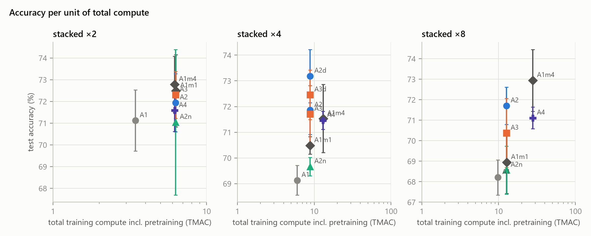
Compute is measured analytically as 3 × (forward multiply-accumulates per image) × (images processed), the usual estimate for forward plus backward. Frozen blocks in greedy pretraining count once for the forward pass. We also record wall-clock time, but report analytic compute because it does not depend on what else the GPU was doing.

4.7Statistics

Differences between groups are computed per seed and summarised with a 95% t-interval over seeds; "p" values are two-sided paired t-tests and, with 4–5 seeds, should be read as rough guides rather than precise probabilities. Rank agreement between block rankings is the Spearman correlation across blocks, with a bootstrap interval over blocks. To tell "the ranking changed" apart from "the ranking is just noisy", we also report the seed-to-seed ceiling: the Spearman correlation between two independent training runs of the same blocks at the same depth. Every population experiment uses two seeds per (block, depth).

4.8Departures from the original plan

• Larger validation and test sets. The initial sketch used 1,000 validation and 1,000 test images. With 1,000 images, one standard error of an accuracy near 70% is about 1.4 percentage points, bigger than most effects we want to measure, so we used 5,000 validation images and the full 10,000-image test set. A practitioner with a truly tiny labelled set would not have 5,000 validation images, so our architecture selection is somewhat more reliable than it would be in a real low-data setting.
• Resolution is not constant across a stack. The original sketch kept resolution fixed inside every block. At 32×32 throughout, our budget would have allowed only a few dozen runs; pooling to 16×16, 8×8 and 4×4 gave a ~4× speed-up and higher accuracy. The consequence is that block copies in later positions operate at a different scale, which is a realistic and arguably more interesting transfer test.
• Search strategies are compared by resampling measured pools (Section 5.8) rather than by running each search end to end. Every candidate in each pool was trained for real, so no accuracy is simulated, but the "searches" are random draws from those pools.
• Population size. 48 blocks rather than 20 to 30.

5Results

Block names read as: P2 = 1×1 expand/project with ratio 2 (noP = none); then the spatial layers (conv3/conv5 = 3×3/5×5 convolution, dw3/dw5 = depthwise-separable); then the activation; then res or plain for the presence of a skip connection.

5.1Phase 1: a population of 48 random blocks

We trained each of the 48 blocks from scratch as a 1-block classifier (two seeds) and, in the same way, stacked 2, 4 and 8 times. Validation accuracy of the 1-block classifiers ranges from 53.2% to 70.8% (mean 62.7%). Seed-to-seed noise is small relative to this spread: the mean standard deviation between two seeds of the same block is 0.44 points at depth 1 and grows to 0.84 points at depth 8. The ranking is therefore reliable (0.98 Spearman between seeds), and the block our search selects, P2_dw5-dw5-dw5_relu_res (OPT), is the best 1-block classifier at 70.8%.

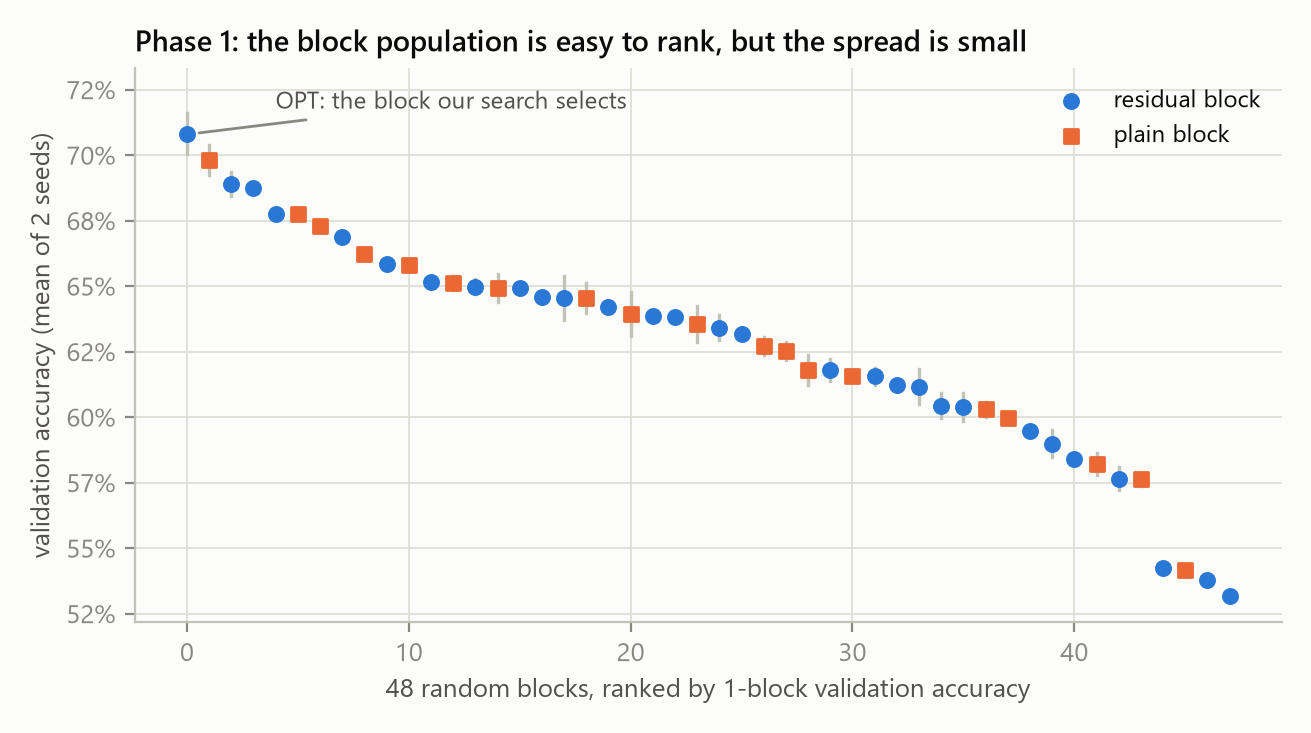
OPT is a residual block with a 1×1 expansion (ratio 2) and three 5×5 depthwise-separable layers. Table 2 shows the eight best 1-block blocks and how they fare when stacked.

Table 2. The eight best blocks by 1-block validation accuracy, and their validation accuracy / rank among the 48 at each stacking depth (mean of 2 seeds).

Block	×1	×2	×4	×8	rank ×1	rank ×2	rank ×4	rank ×8	params (×1)
P2_dw5-dw5-dw5_relu_res	70.8%	70.7%	69.4%	68.3%	1	4	12	17	23,018
P2_dw5-dw5-conv3_gelu_plain	69.8%	69.6%	64.7%	41.7%	2	11	39	46	54,186
P2_dw3-dw3-dw3_relu_res	68.9%	70.9%	68.7%	67.3%	3	2	14	22	19,946
P2_dw5-dw5_relu_res	68.8%	70.4%	69.5%	68.5%	4	5	9	16	17,194
P1_conv5-conv3_gelu_res	67.8%	69.8%	68.8%	68.7%	5	10	13	15	38,378
P1_dw5-conv3-conv5_gelu_plain	67.7%	67.5%	60.7%	39.6%	6	22	46	47	40,266
noP_conv3-conv5-dw5_gelu_plain	67.3%	69.6%	66.8%	59.7%	7	12	26	37	38,090
noP_dw3-conv5-conv3_gelu_res	66.9%	71.0%	70.1%	70.7%	8	1	5	4	37,578

5.2Does small-block quality predict stacked quality? (H2b)

Not beyond two blocks. Figure 4 plots 1-block accuracy against stacked accuracy. The rank correlation is 0.73 for ×2 (95% bootstrap interval 0.57 to 0.83) but falls to 0.06 (-0.22 to 0.33) at ×4 and -0.08 (-0.35 to 0.19) at ×8. This is not noise: two independent training runs of the same blocks at the same depth agree with a Spearman correlation of 0.94, 0.93 and 0.97, so the loss of agreement is a real change in which blocks are good, not an artefact of unreliable measurement. Using different seeds for the small and large networks (so no shared noise) gives the same picture (0.72, 0.04, -0.09).

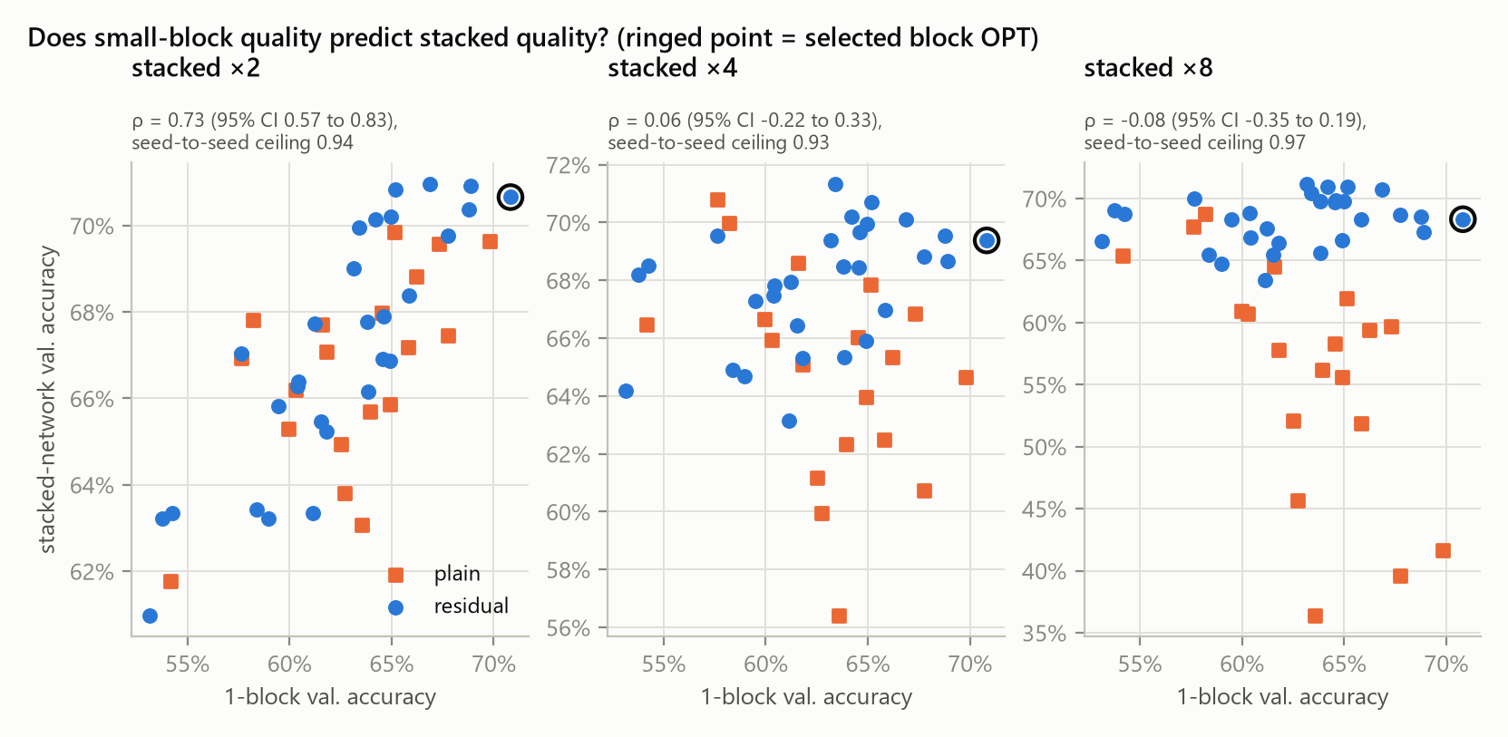
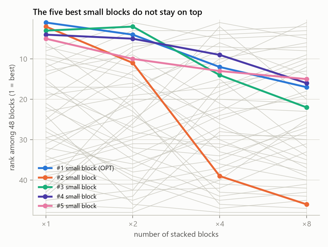
For our own selected block, the effect is concrete: OPT is rank 1 of 48 with one block, rank 4 at ×2, rank 12 at ×4 and rank 17 at ×8 (Figure 5). The five best 1-block blocks share 0 members with the five best ×4 stacks and 0 with the five best ×8 stacks. Picking the best 1-block block costs 2.0 validation points relative to the best ×4 stack and 2.9 points relative to the best ×8 stack. OPT is still a good block (it is +4.9 points above the population mean at ×8), but, as the next section shows, that is largely for a reason unrelated to its 1-block score.

5.3Why the ranking breaks: trainability, not "better features"

The explanation is visible in Figure 6. With residual connections blocks keep improving with depth (mean 68.2% at ×8). Plain blocks improve from ×1 to ×2 and then deteriorate, reaching 56.0% at ×8 on average (19 blocks; Mann-Whitney p<0.001), and several fall below 45%. At depth 1 the two groups are indistinguishable (62.5% vs 63.0%, p = 0.74), so the 1-block score cannot see the property that will matter later. Deep plain networks are hard to train from scratch in 30 epochs, a known problem that skip connections solve.^{22, 23}

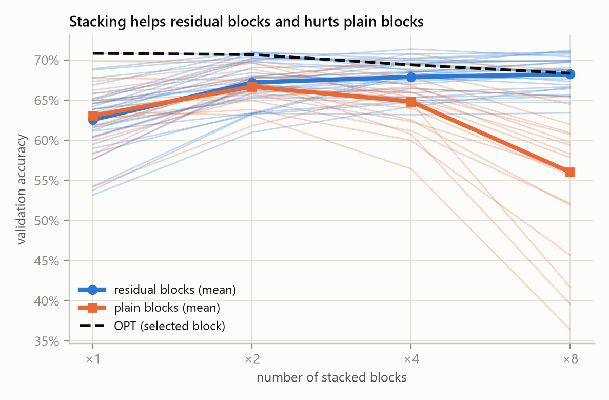
A single bit, has a skip connection, is a better predictor of ×8 accuracy (Spearman 0.75) than the full 1-block accuracy is (-0.08). Restricting attention to the 29 residual blocks shows that architecture transfer is not zero, but it decays with depth: Spearman 0.85 at ×2, 0.50 at ×4 (p = 0.006) and 0.27 at ×8 (p = 0.16, not significant), against seed-to-seed ceilings of 0.94, 0.86 and 0.91.

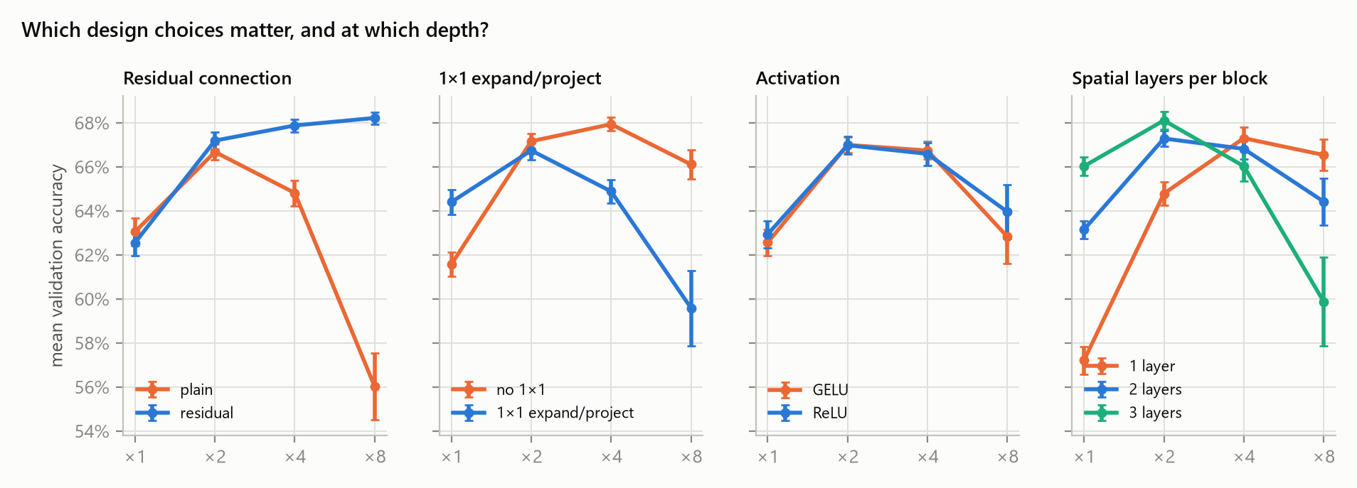
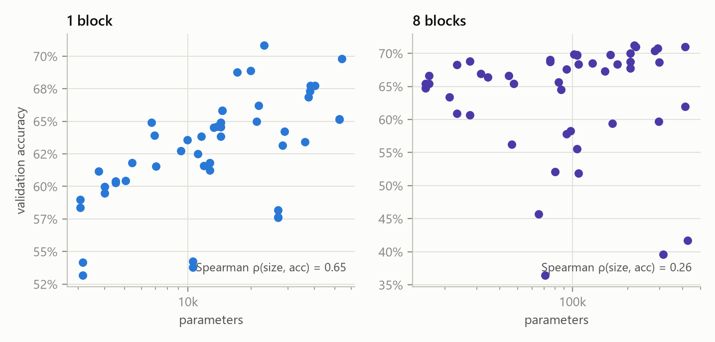
Other design choices show the same pattern of "good alone, costly when repeated". Blocks with three spatial layers are best as 1-block classifiers (66.0% on average) but, repeated eight times, give 59.9%; one-layer blocks are the opposite (57.2% alone, 66.5% at ×8). A 1-block network rewards capacity per block, whereas an 8-block network is rewarded for being easy to optimise as a composition. Parameter count alone does not explain it: block size correlates with 1-block accuracy (0.65) but much less with ×8 accuracy (0.26, Figure 8).

5.4Does pretraining help when stacking? (H1) preliminary: 4 seeds

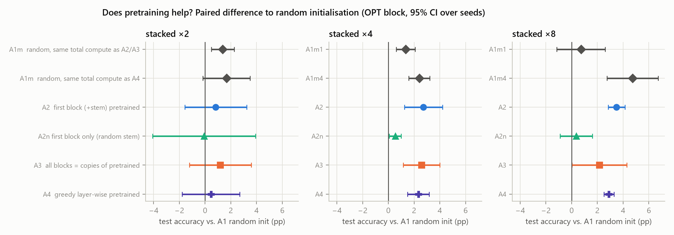
We trained the OPT block as a 1-block classifier on the 5,000 training images and used it to initialise stacks of 2, 4 and 8 blocks (Figure 1). Figure 9 and Table 3 show the test-accuracy gain over random initialisation (A1), paired by seed.

Table 3. Test accuracy (%, mean ± 95% interval over 4 seeds) of the OPT block for each initialisation. “vs A1”: paired difference to random init (percentage points). “vs match”: difference to the compute-matched random-init control A1m1 (same total training compute including pretraining). A4 should be compared with A1m4.

Initialisation	×2	vs A1	vs match	×4	vs A1	vs match	×8	vs A1	vs match
A1 random init	71.1 ± 1.4	–	–	69.1 ± 0.6	–	–	68.2 ± 0.9	–	–
A1m random, compute-matched to A2/A3	72.5 ± 1.7	+1.4	–	70.5 ± 0.3	+1.4	–	68.9 ± 1.5	+0.7	–
A1m random, compute-matched to A4	72.8 ± 1.3	+1.7	–	71.5 ± 1.3	+2.4	–	72.9 ± 1.5	+4.7	–
A2 first block + stem pretrained	71.9 ± 1.3	+0.8	−0.5	71.9 ± 1.0	+2.7	+1.4	71.7 ± 0.9	+3.5	+2.8
A2n first block only	71.0 ± 3.3	−0.1	−1.4	69.7 ± 0.4	+0.5	−0.8	68.6 ± 1.2	+0.4	−0.4
A3 all blocks copied	72.3 ± 1.1	+1.2	−0.2	71.7 ± 1.1	+2.6	+1.2	70.4 ± 1.7	+2.2	+1.4
A4 greedy layer-wise	71.6 ± 1.0	+0.5	−0.9	71.5 ± 0.4	+2.3	+1.0	71.1 ± 0.5	+2.9	+2.2
A2d first block, extra data	–	–	–	73.2 ± 1.0	+4.1	+2.7	–	–	–
A3d all copies, extra data	–	–	–	72.5 ± 1.0	+3.3	+2.0	–	–	–

Against plain random initialisation, pretraining helps at depths 4 and 8: stem-and-first-block transfer (A2) gains +2.7 points at ×4 and +3.5 at ×8; copying the block everywhere (A3) is similar (+2.6 and +2.2) and greedy layer-wise pretraining (A4) too. At ×2 the gains are small and not clearly different from zero (+0.8 for A2). Pretraining is therefore not harmful here; in particular we did not see the warm-start penalty reported for other settings.¹⁹

But most of this is "more training", not "better start". Pretraining on the same 5,000 images costs compute. When random initialisation is simply trained for as many epochs as the pretrained variant's total compute (A1m1), it recovers a large part of the gain: +1.4 at ×2, +1.4 at ×4, +0.7 at ×8. Relative to this fair control, A2 and A3 are no better at ×2 (−0.5) but better at ×4 (+1.4) and ×8 (+2.8), so at equal compute pretraining does deliver a modest benefit for deeper stacks. The picture reverses when random initialisation is given more: greedy layer-wise pretraining is expensive (about 2.2× the compute of A2 at ×8) and its matched control (A1m4, 85 epochs at ×8) is better than A4 by 1.8 points at ×8 (A4 − A1m4 = −1.8), and no better at ×2 (−1.2) or ×4 (−0.1). The best single number at ×8 comes from plain random initialisation trained long enough.

The stem matters. Transferring the block but not the stem (A2n) gives essentially nothing (+0.5 at ×4, +0.4 at ×8). The pretrained block was trained against a particular set of stem features; with a random stem its weights are mismatched, and the benefit disappears. "Pretrained block" results that transfer only the block therefore understate (or miss) what transfer can do.

Copying one block everywhere works nearly as well as pretraining each position. A3 (identical copies in every position) is statistically close to A2 and to A4 despite being the variant we considered least likely to work, since a block pretrained at 16×16 now runs at 8×8 and 4×4. This echoes the success of stacking copies in language-model growth,^{17, 18} though here the effect is small.

Extra data is a real advantage. Pretraining on 5,000 different images (A2d, A3d) gains +4.1 / +3.3 points at ×4, about +1.3 points more than the same-data version. Some of what same-data pretraining captures is simply more optimisation; extra data adds information.

Convergence (H1a)

Pretrained starts are far ahead early: after the first epoch the validation accuracy is 50% for A2 against 24% for random init at ×4 (Figure 10), and A2 reaches 95% of the random-init final accuracy after 15 epochs instead of 21. The early dip around epoch 2 is the learning-rate warm-up disturbing the pretrained weights. By the end the curves converge, which is why the advantage in final accuracy is much smaller than the advantage in speed.

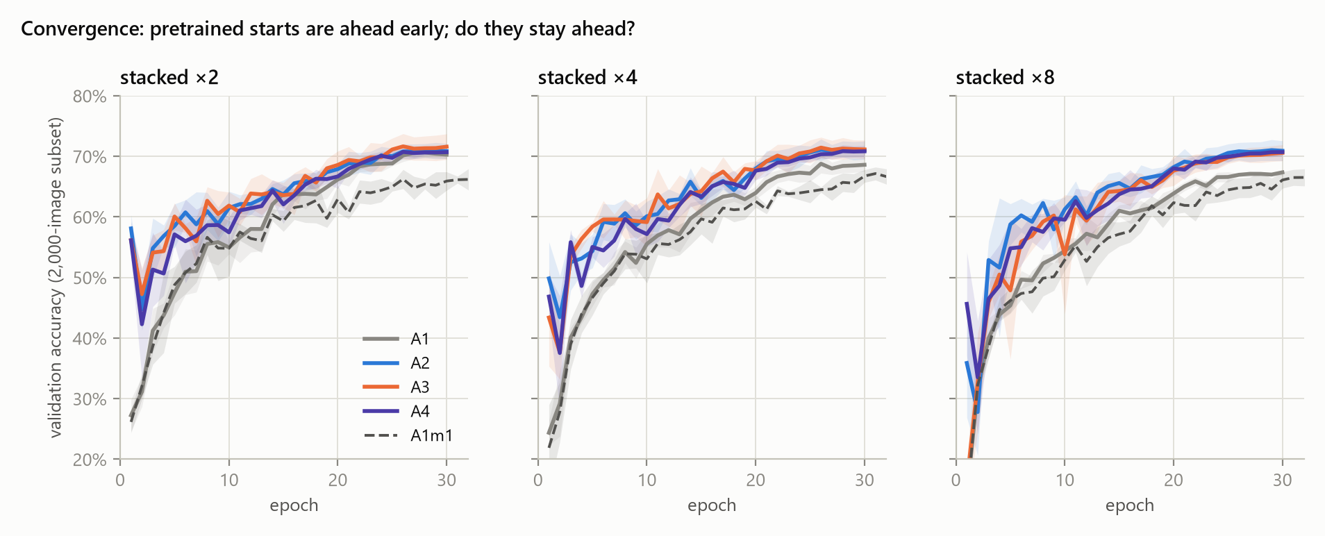
Every configuration overfits strongly: training accuracy is 90–99% against 69–73% test accuracy, a gap of 20–27 points that varies little between variants. This is the low-data regime the experiment was designed to probe.

5.5Is pretraining more useful for an optimised block than a random one? (H3) exploratory: 2 seeds

We repeated the main comparison for two further blocks: noP_conv5-conv5_gelu_plain (RND1, a uniform random draw) and P2_dw5-dw5-conv3_gelu_plain (OPT2, the runner-up in the 1-block ranking), with two seeds each. Both turned out to be plain blocks, so this comparison mixes “optimised vs random” with “plain vs residual”, and two seeds give only a rough view. Gain of A2 / A3 over random initialisation (percentage points), with the compute-matched control A1m1 in brackets:

Table 4. Test-accuracy gain over random initialisation (pp) for different blocks. n = 4 seeds for OPT, 2 for the others.

Block	×4: A2	×4: A3	×4: A1m1	×8: A2	×8: A3	×8: A1m1
OPT P2_dw5-dw5-dw5_relu_res	+2.7	+2.6	+1.4	+3.5	+2.2	+0.7
OPT2 P2_dw5-dw5-conv3_gelu_plain	+3.9	+4.7	+2.2	+8.7	+6.9	+5.6
RND1 noP_conv5-conv5_gelu_plain	−0.1	−0.1	+1.7	+4.4	+5.3	+3.4

The pattern does not support a simple interaction in either direction. The optimised block (OPT) gains +2.7 (A2) at ×4. The plain runner-up gains more (+3.9), the random plain block gains nothing (−0.1). At ×8, where plain blocks are hard to train from scratch, pretraining helps both plain blocks by 4 to 9 points, but the intervals are very wide: for OPT2 one random-init seed collapsed, so pretraining acts partly as a stabiliser for blocks that train poorly. Our reading is that pretraining helps most where random initialisation struggles, rather than where the block is “optimised”. A clean test needs random blocks drawn from the residual-only part of the space.

5.6Does pretraining only help with very little data? OPT block, ×4, 2 seeds

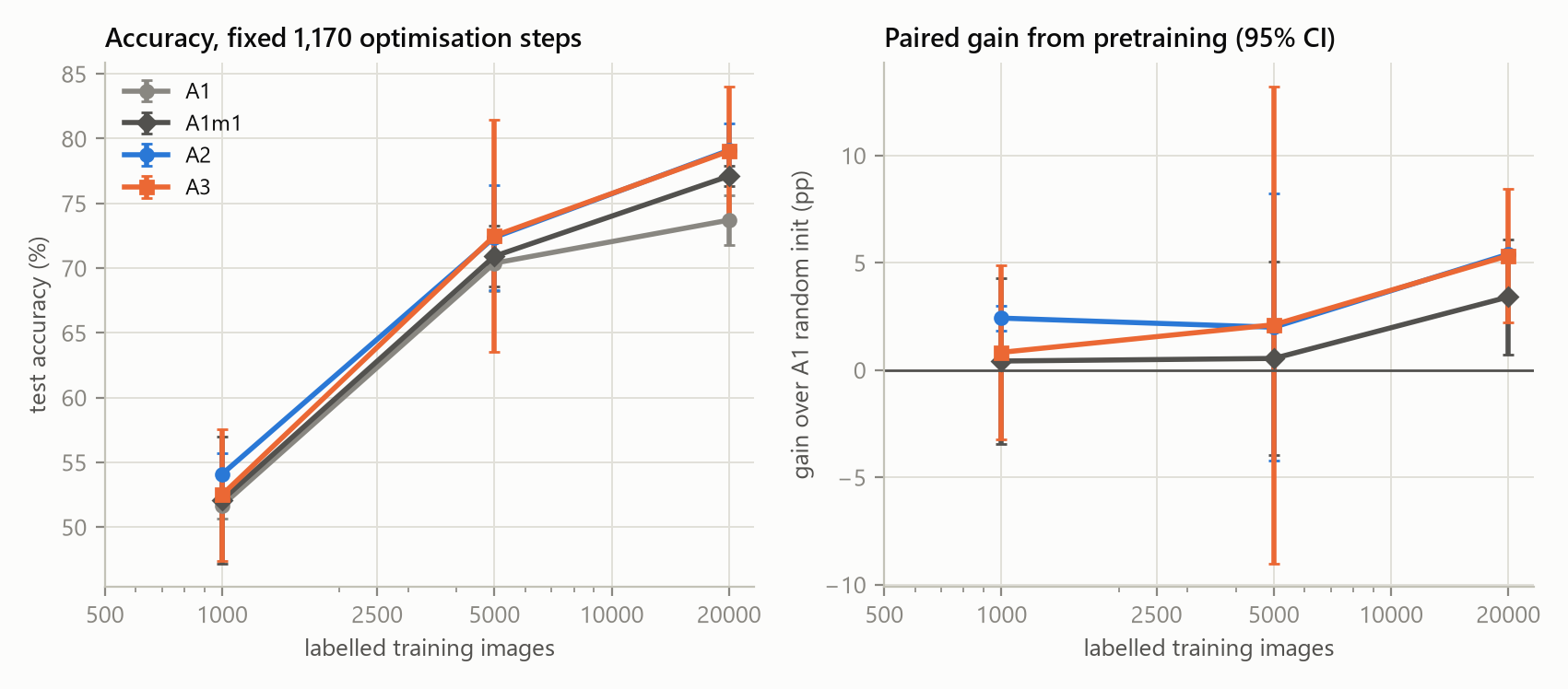
We varied the labelled training set from 1,000 to 20,000 images (100, 500, 2,000 per class), keeping the number of optimisation steps fixed at 1,170 so that compute is comparable across sizes (30 epochs at 5,000 images, about 7 at 20,000, 167 at 1,000). The block is pretrained on the same subset it is fine-tuned on.

Table 6. Test accuracy (%, mean of 2 seeds) of the OPT block stacked ×4 for different amounts of labelled data.

Labelled images	A1 random	A1m random, matched compute	A2 first block	A3 all copies
1,000	51.7	52.1	54.1	52.5
5,000	70.4	70.9	72.4	72.5
20,000	73.7	77.1	79.1	79.0

The expectation that pretraining mainly helps in the very-low-data regime is not what we see. The gain of A2 over random initialisation is +2.4 points at 1,000 images, +2.0 at 5,000 and +5.4 at 20,000; against the compute-matched control the gains are +2.0, +1.5 and +2.0. A likely reason is our fixed-steps protocol: at 20,000 images the random-init network sees each image only about seven times and is under-trained, which gives a head start more to work with. We therefore read this as “pretraining does not need tiny data to help” rather than as evidence that it helps more with more data. With two seeds and three sizes it is a coarse check.

5.7Searching small blocks vs searching stacks directly (H2a, H2c)

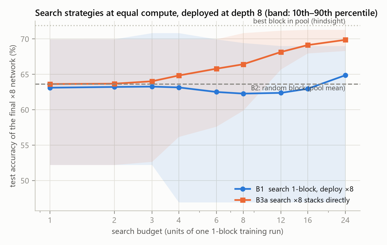
We simulated compute-matched searches by resampling from the measured pools of 48 trained blocks (Section 4.8). A search draws blocks in random order until a compute budget is exhausted, picks the best by validation accuracy and is scored on the test accuracy of an independent run of the chosen block. Budgets are in units of one 1-block training run. B1 evaluates blocks as 1-block networks and deploys the winner stacked; B3a evaluates each candidate directly as a stack of the deployment depth (so fewer candidates fit in the budget: about 2.1 units each at ×4, 3.4 at ×8); B2 picks a random block.

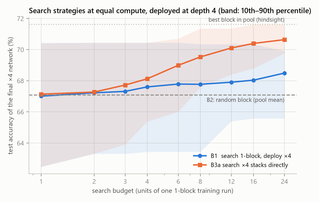
The result is one-sided. At deployment depth 4, B1 beats a random block only slightly (at 24 units: 68.5% against 67.1% for B2), while direct search (B3a) reaches 70.6%. At the same budget of 16 units the simulated B1 wins against B3a in only 14% of paired trials. At depth 8 the small-block search is worse than picking a random block for budgets of 4 to 16 units (62.3% at 8 units against 63.6% random), whereas direct search climbs to 69.9%. The reason is the correlation reported in Section 5.2: the validation accuracy of 1-block networks is nearly uninformative about stacked test accuracy (Spearman 0.07 at ×4), whereas validation accuracy of the stack is highly informative (0.94). So H2c (small-block search is more compute-efficient) is not supported: a 1-block evaluation is cheaper per candidate, but the extra candidates it buys are scored by a poor proxy.

We did not run the planned third strategy (searching over heterogeneous networks where every position has its own block); it is left for future work.

Caveat. The pool contains only 48 blocks, and the random-block baseline is the pool mean. Our search space includes many plain blocks that fail at depth, which makes random selection look worse than in a space designed by hand and makes any proxy that detects trainability valuable; a space restricted to residual blocks would shrink the gaps.

5.8Stacking versus widening OPT block, 2 seeds

For the OPT block we trained a grid of depths (1, 2, 4, 8 blocks) and widths (16, 32, 64 channels), two seeds each, from random initialisation. Test accuracy (%):

Table 5. Test accuracy (%) of the OPT block over depth and width (mean of 2 seeds).

blocks N	C = 16	C = 32	C = 64
1	65.9	70.2	73.8
2	66.0	70.9	74.0
4	64.6	69.1	70.9
8	64.0	68.6	70.0

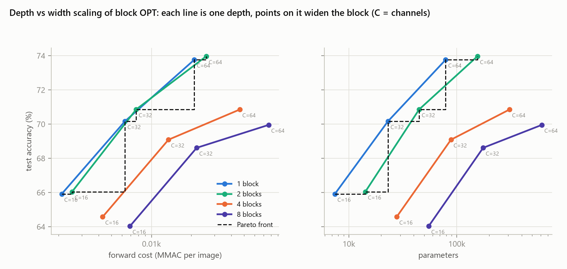
Width wins. At matched cost, shallow wide networks beat deep narrow ones in every one of the 5 matched pairs we could form (mean −5.6 points for the deeper network; for example 8 blocks at 32 channels, 68.6%, against 1 block at 64 channels, 73.8%, at about the same cost). The Pareto front consists only of networks with one or two blocks. Even at fixed width, adding blocks beyond two lowered accuracy in our 30-epoch budget (32 channels: 70.2% with one block, 70.9% with two, 69.1% with four, 68.6% with eight). This agrees with the observation that wide networks can beat deep ones at matched cost,²⁰ and is consistent with the trainability story of Section 5.3: with a fixed short training budget on 5,000 images, depth is harder to exploit than width. It is also consistent with the weak rank transfer of Section 5.2: a block designed to be stacked many times may simply not be what a small-data problem needs. Caveats: one block, two seeds, three widths, a fixed training budget, and widths beyond 64 were not tried.

6What we expected and what we found

Table 7. Expectations written down before the experiments versus observed results.

Question	Expected	Observed
H1a first-block pretraining converges faster	Moderate: yes	As expected. Far higher accuracy in the first epochs; reaches the random-init final level 3–8 epochs sooner.
H1b pretraining improves final accuracy	Uncertain	Mixed. +2 to +3.5 points over plain random init at ×4/×8, but compute-matched random training recovers about half of it at ×4 and all of it at ×2.
H1c effect changes with depth	Uncertain	Yes. Small at ×2, larger at ×4 and ×8.
H1d copying one block everywhere helps	Low	Surprise (mild). It helps nearly as much as position-specific pretraining.
H2a optimised block beats random blocks	Moderate: yes	Yes, but for the wrong reason. OPT is residual, and residual blocks beat plain ones at depth.
H2b small-block ranking predicts stacked ranking	Uncertain	No beyond ×2. ρ = 0.73, 0.06, −0.08 at ×2/×4/×8.
H2c small-block search is more compute-efficient	Moderate: yes	No. Direct search at deployment depth wins at equal compute.
H3 pretraining interacts with block quality	Open	Inconclusive. No consistent interaction; the biggest gains were for blocks that train poorly. Confounded and only 2 seeds.
Pretraining only helps with tiny data	(listed as possible surprise)	Not observed. Gains were not larger at 1,000 images.
Width vs depth	(open)	Width wins at matched cost for this block.

7What surprised us

8Limitations

• One dataset, one small-data regime, one network family. Findings about trainability at depth in particular depend on our plain (non-residual) blocks, on the 30-epoch budget and on BatchNorm without special initialisation.
• Few seeds. The main pretraining comparison uses 4 seeds of one block; the interaction, scaling and data-size experiments use 2. Intervals are wide, p-values are rough guides, and differences below about 1 point are not supported.
• Search is simulated by resampling from 48 trained blocks, not run end to end with an adaptive algorithm, and the planned heterogeneous full-network search was not run.
• Our "optimised block" is the best of 48 random draws by a 1-block proxy, not the result of a sophisticated search.
• The comparison blocks were both plain, so the optimised-versus-random interaction test is confounded with residual-versus-plain.
• Same-data pretraining adds no information. With large external pretraining data the conclusions about weight transfer may differ.
• Validation set size. We selected on 5,000 images, more than a realistic low-data user would have, so real selection would be noisier than shown.
• Dataset-size sweep fixes the number of steps, which favours pretraining at larger sizes.

9Conclusions and practical guidance

1. Do not trust a shallow proxy to rank blocks for deep stacks. It was reliable to two blocks and not beyond. Evaluate candidates at (or near) the depth you intend to deploy, or at least include a trainability check such as a skip connection.
2. If you must use a small-block search, restrict the space to blocks that are known to stack (for example residual blocks); the 1-block ranking was most informative within that group.
3. Pretraining on your own small dataset is a speed-up and a modest regulariser, not magic. Compare against random init with the same total compute before concluding it helps. If you transfer weights, transfer the stem together with the block.
4. Copy-paste stacking (one pretrained block copied into every position) was nearly as good as separately pretrained blocks and far cheaper to produce.
5. With 5,000 images, try widening before deepening. Our best networks had one or two wide blocks.

10Frequently asked questions

Does pretraining a small block help when you stack it into a deeper network?

In our CIFAR-10 low-data experiment, yes versus plain random initialisation (about +2 to +3.5 points at 4 and 8 blocks) and with much faster early convergence. But a randomly initialised network trained for the same total compute recovered a large part of that gain, so much of the benefit was extra optimisation rather than a better starting point.

Is the best small block still the best when you stack it many times?

Not reliably. Rankings of 48 random blocks agreed well between 1 and 2 blocks (Spearman 0.73), but not between 1 and 4 or 8 blocks (0.06 and −0.08). The best 1-block design ranked 17th of 48 at 8 blocks.

Why do some blocks fail when stacked?

Mostly because they have no skip connection. Plain blocks averaged 56% validation accuracy at 8 blocks against 68% for residual blocks, although they were indistinguishable at 1 block.

Is it cheaper to search for a small block and stack it than to search the full network?

Per candidate, yes; in total, no. At equal compute, evaluating candidates at the deployment depth gave better final networks, because the cheap 1-block score was an almost uninformative proxy.

Should I copy pretrained weights into every layer?

In our experiment, copying one pretrained block into every position performed nearly as well as pretraining each position separately, and was much cheaper. Copying only the block and not the stem gave no benefit.

Is it better to make a network deeper or wider?

For our optimised block on 5,000 CIFAR-10 images with a 30-epoch budget, wider and shallower won at every matched cost: one or two blocks with 64 channels beat eight blocks with 32 channels by about 5 points.

Does pretraining only help when there is very little labelled data?

Not in our test. Gains over random initialisation were similar or larger with 20,000 labelled images than with 1,000, although our fixed-number-of-steps protocol favours pretraining at larger sizes.

11Reproducibility

All experiments ran on a single NVIDIA GTX 1070 using PyTorch with the splits, seeds and hyper-parameters stated in Section 4. Results for every individual run (validation and test accuracy, learning curves, parameters, compute) are stored as JSON lines, and the analysis scripts regenerate every figure and table in this paper from those files. Code and raw results to be linked here.

Statement on AI assistance

The experiments were designed, run and written up by the author together with Claude (Anthropic), an AI assistant, which wrote the code and the first draft of the text. The numbers come from the runs described; the author is responsible for the content.

References

1. Zoph, B., Vasudevan, V., Shlens, J., Le, Q. V. (2018). Learning Transferable Architectures for Scalable Image Recognition. CVPR. arXiv:1707.07012
2. Real, E., Aggarwal, A., Huang, Y., Le, Q. V. (2019). Regularized Evolution for Image Classifier Architecture Search. AAAI. arXiv:1802.01548
3. Liu, H., Simonyan, K., Yang, Y. (2019). DARTS: Differentiable Architecture Search. ICLR. arXiv:1806.09055
4. Elsken, T., Metzen, J. H., Hutter, F. (2019). Neural Architecture Search: A Survey. JMLR 20(55). jmlr.org
5. Krizhevsky, A. (2009). Learning Multiple Layers of Features from Tiny Images. Technical report, University of Toronto. CIFAR-10 page
6. Li, L., Talwalkar, A. (2019). Random Search and Reproducibility for Neural Architecture Search. UAI. arXiv:1902.07638
7. Yang, A., Esperança, P. M., Carlucci, F. M. (2020). NAS evaluation is frustratingly hard. ICLR. arXiv:1912.12522
8. Yu, K., Sciuto, C., Jaggi, M., Musat, C., Salzmann, M. (2020). Evaluating the Search Phase of Neural Architecture Search. ICLR. arXiv:1902.08142
9. Ying, C., Klein, A., Real, E., Christiansen, E., Murphy, K., Hutter, F. (2019). NAS-Bench-101: Towards Reproducible Neural Architecture Search. ICML. arXiv:1902.09635
10. Dong, X., Yang, Y. (2020). NAS-Bench-201: Extending the Scope of Reproducible Neural Architecture Search. ICLR. arXiv:2001.00326
11. Mellor, J., Turner, J., Storkey, A., Crowley, E. J. (2021). Neural Architecture Search without Training. ICML. arXiv:2006.04647
12. Bengio, Y., Lamblin, P., Popovici, D., Larochelle, H. (2006). Greedy Layer-Wise Training of Deep Networks. NIPS. papers.nips.cc
13. Erhan, D., Bengio, Y., Courville, A., Manzagol, P.-A., Vincent, P., Bengio, S. (2010). Why Does Unsupervised Pre-training Help Deep Learning? JMLR 11. jmlr.org
14. Yosinski, J., Clune, J., Bengio, Y., Lipson, H. (2014). How transferable are features in deep neural networks? NIPS. arXiv:1411.1792
15. Belilovsky, E., Eickenberg, M., Oyallon, E. (2019). Greedy Layerwise Learning Can Scale to ImageNet. ICML. arXiv:1812.11446
16. Chen, T., Goodfellow, I., Shlens, J. (2016). Net2Net: Accelerating Learning via Knowledge Transfer. ICLR. arXiv:1511.05641
17. Gong, L., He, D., Li, Z., Qin, T., Wang, L., Liu, T.-Y. (2019). Efficient Training of BERT by Progressively Stacking. ICML. PMLR 97
18. Du, W., Luo, T., Qiu, Z., Huang, Z., Shen, Y., Cheng, R., Guo, Y., Fu, J. (2024). Stacking Your Transformers: A Closer Look at Model Growth for Efficient LLM Pre-Training. NeurIPS. neurips.cc
19. Ash, J. T., Adams, R. P. (2020). On Warm-Starting Neural Network Training. NeurIPS. arXiv:1910.08475
20. Zagoruyko, S., Komodakis, N. (2016). Wide Residual Networks. BMVC. arXiv:1605.07146
21. Tan, M., Le, Q. V. (2019). EfficientNet: Rethinking Model Scaling for Convolutional Neural Networks. ICML. arXiv:1905.11946
22. He, K., Zhang, X., Ren, S., Sun, J. (2016). Deep Residual Learning for Image Recognition. CVPR. arXiv:1512.03385
23. Balduzzi, D., Frean, M., Leary, L., Lewis, J. P., Ma, K. W.-D., McWilliams, B. (2017). The Shattered Gradients Problem: If resnets are the answer, then what is the question? ICML. arXiv:1702.08591
24. Ioffe, S., Szegedy, C. (2015). Batch Normalization: Accelerating Deep Network Training by Reducing Internal Covariate Shift. ICML. arXiv:1502.03167
25. Howard, A. G., et al. (2017). MobileNets: Efficient Convolutional Neural Networks for Mobile Vision Applications. arXiv:1704.04861
26. Sandler, M., Howard, A., Zhu, M., Zhmoginov, A., Chen, L.-C. (2018). MobileNetV2: Inverted Residuals and Linear Bottlenecks. CVPR. arXiv:1801.04381
27. Loshchilov, I., Hutter, F. (2017). SGDR: Stochastic Gradient Descent with Warm Restarts. ICLR. arXiv:1608.03983